Multilevel Summation Method
Algorithmic Details
MSM approximates the Coulombic potential energy for a system of $N$ particles having position $\vec{r}_i$ and charge $q_i$, \begin{equation} U(\vec{r}_1,\vec{r}_2,\dots,\vec{r}_N) = \frac{1}{2} \sum_{i=1}^N \sum_{j\neq i} q_i q_j\, k(\vec{r}_i,\vec{r}_j), \qquad k(\vec{r},\vec{r}') = \frac{1}{|\vec{r}'-\vec{r}|}, \label{eq:potential} \end{equation} by splitting the interaction kernel $k$ into the sum of a short-range part $k_0$ smoothly truncated at cutoff distance $a$ and slowly varying parts $k_1, k_2, \dots, k_{L-1}, k_L$ smoothly truncated at cutoff distances $2a, 4a, \dots, 2^{L-1}a, \infty$, respectively, \begin{equation*} k(\vec{r},\vec{r}') = k_0(\vec{r},\vec{r}') + k_1(\vec{r},\vec{r}') + \dots + k_{L-1}(\vec{r},\vec{r}') + k_L(\vec{r},\vec{r}'). \end{equation*} The splitting can be defined systematically in terms of a single unparameterized softening function $\gamma(R)$ that softens $1/R$ for $R\leq 1$, \begin{align} \begin{split} k_0(\vec{r},\vec{r}') &= \frac{1}{|\vec{r}'-\vec{r}|} - \frac{1}{a}\gamma\Bigl(\frac{|\vec{r}'-\vec{r}|}{a}\Bigr), \\ k_l(\vec{r},\vec{r}') &= \frac{1}{2^{l-1}a}\gamma\Bigl(\frac{|\vec{r}'-\vec{r}|}{2^{l-1}a}\Bigr) - \frac{1}{2^{l}a}\gamma\Bigl(\frac{|\vec{r}'-\vec{r}|}{2^{l}a}\Bigr), \quad l=1,2,\dots,L-1, \\ k_L(\vec{r},\vec{r}') &= \frac{1}{2^{L-1}a}\gamma\Bigl(\frac{|\vec{r}'-\vec{r}|}{2^{L-1}a}\Bigr). \end{split} \label{eq:splitting} \end{align} The slowly varying parts are interpolated from grids of spacing $h, 2h, \dots, 2^{L-2}h, 2^{L-1}h$, respectively, for which interpolation operators $\Int_l$ are defined in terms of interactions between grid point positions $\vec{r}_m^l = (x_m^l,y_m^l,z_m^l)\T$ and their corresponding nodal basis functions $\phi_m^l$, \begin{equation} \Int_l \, k_l(\vec{r},\vec{r}') = \sum_m \sum_n \phi_m^l(\vec{r}) \, k_l(\vec{r}_m^l,\vec{r}_n^l) \, \phi_n^l(\vec{r}'), \quad l=1,2,\dots,L. \label{eq:interp} \end{equation} The nodal basis functions can be defined in terms of a single dimensionless basis function $\Phi$, $$ \phi_m^l(\vec{r}) = \Phi\Bigl(\frac{x-x_m^l}{2^{l-1} h}\Bigr) \Phi\Bigl(\frac{y-y_m^l}{2^{l-1} h}\Bigr) \Phi\Bigl(\frac{z-z_m^l}{2^{l-1} h}\Bigr). $$ Interpolation by piecewise polynomials of degree $p$ provides local support for $\Phi$ with stencil size $p+1$. Continuous forces necessary for stable dynamics are produced from a continuously differentiable $\Phi$ and sufficient continuity from $\gamma$. The approximation is made efficient by nesting the interpolation between levels, \begin{equation} k(\vec{r},\vec{r}') \approx \biggl( k_0 + \Int_1 \Bigl( k_1 + \Int_2 \bigl( k_2 + \cdots \Int_{L-1} ( k_{L-1} + \Int_L k_L ) \cdots \bigr) \Bigr) \biggr) (\vec{r},\vec{r}'). \label{eq:multilevel} \end{equation}
The CHARMM force field prescribes a cutoff distance of $a=12\Ang$ for calculating van der Waals forces, which we adopt for the efficiency of calculating all short-range non-bonded interactions with the same cutoff distance. The choice of grid spacing $h=2.5\Ang$, which is a little bit larger than the interatomic spacing, works effectively in practice. The computational work per grid point is bounded by a constant, and the number of grid points is reduced by about a factor of $1/8$ at each successive level. The computational cost of MSM is $O\bigl((p^3 + (a/h)^3)N\bigr)$, and analysis of the error shows an asymptotic bound of the form $$ \text{potential energy error} %= O\biggl(\frac{1}{a}\Bigl(\frac{h}{a}\Bigr)^p\biggr), = O\Bigl(\frac{h^p}{a^{p+1}}\Bigr), \quad \text{force error} %= O\biggl(\frac{1}{a^2}\Bigl(\frac{h}{a}\Bigr)^{p-1}\biggr), = O\Bigl(\frac{h^{p-1}}{a^{p+1}}\Bigr). $$ Experiments in the present study test $C^1$ cubic interpolation ($p=3$) with $C^2$ splitting, for which the functional forms of $\Phi$ and $\gamma$, given in the following section, are among the lowest order choices that produce continuous forces.
The potential energy is approximated by substituting Eqs.\eqref{eq:multilevel} and \eqref{eq:splitting} into Eq.\eqref{eq:potential}, \begin{equation} U \approx U^{\text{MSM}} = \frac{1}{2} \sum_{i=1}^N \sum_{j\neq i} q_i q_j k_0(\vec{r}_i,\vec{r}_j) + \frac{1}{2} \sum_{i=1}^N q_i e_i^{\text{long}} - \frac{1}{2} \sum_{i=1}^N q_i^2 \frac{1}{a} \gamma(0), \label{eq:mlpot} % mlpot = multilevel potential \end{equation} where the first summation is the exact short-range part, the second summation is the approximate long-range part, and the final summation removes the excluded self-interactions from the long-range part. The $e_i^{\text{long}}$ long-range atomic potential is \begin{equation} e_i^{\text{long}} = \sum_{j=1}^N \Int_1 \Bigl( k_1 + \Int_2 \bigl( k_2 + \cdots \Int_{L-1} ( k_{L-1} + \Int_L k_L ) \cdots \bigr) \Bigr) (\vec{r}_i,\vec{r}_j)\,q_j. \label{eq:elong} \end{equation}
The short-range part of Eq.\eqref{eq:mlpot} simply evaluates all atom pair interactions within the cutoff distance $a$. The algorithm for $e_i^{\text{long}}$ in Eq.\eqref{eq:elong} is made efficient by factoring the interpolation operator in Eq.\eqref{eq:interp}, calculating at each grid point intermediate charges $q_m^l$ and potentials $e_m^l$. The order of the calculation is the following: \begin{align} \text{anterpolation:}& \quad q_{m}^1 = \sum_j \phi_{m}^1(\vec{r}_j) \, q_j, \label{eq:anterpolation} \\ \text{restriction:}& \quad q_{m}^{l+1} = \sum_{n} \phi_{m}^{l+1}(\vec{r}_{n}^l) \, q_{n}^l, \quad l=1,2,\dots,L-1, \label{eq:restriction} \\ \text{grid cutoff calculation:}& \quad e_{m}^{l,\text{cutoff}} = \sum_{n} k_{l}(\vec{r}_{m}^l,\vec{r}_{n}^l) \, q_{n}^l, \quad l=1,2,\dots,L-1, \label{eq:gridcutoff} \\ \text{top level grid calculation:}& \quad e_{m}^{L} = \sum_{n} {k}_{L}(\vec{r}_{m}^{L},\vec{r}_{n}^{L}) \, q_{n}^{L}, \label{eq:toplevel} \\ \text{prolongation:}& \quad e_{m}^{l,\text{long}} = \sum_{n} \phi_{n}^{l+1}(\vec{r}_{m}^l) \, e_{n}^{l+1}, \quad l=L-1,\dots,2,1, \label{eq:prolongation} \\ &\quad e_{m}^l = e_{m}^{l,\text{cutoff}} + e_{m}^{l,\text{long}}, \quad l=L-1,\dots,2,1, \nonumber %\label{eq:confluence} \\ \text{interpolation:}& \quad e_i^{\text{long}} = \sum_{m} \phi_{m}^1(\vec{r}_i) \, e_{m}^1. \label{eq:interpolation} \end{align} The diagram in Figure 1 depicts the computational steps and their dependencies. The bottom--left shows the atom positions and charges, and the calculated potentials and forces are on the bottom--right. The gridded charges are calculated for each level moving up the left side, and the gridded potentials are calculated moving down the right side. The horizontal arrows represent the calculation of the short-range part along the bottom and the grid cutoff calculations for each grid level, all of which collectively require the majority of the computational effort. Forces are obtained analytically by taking the negative gradient of Eq.\eqref{eq:mlpot}, \begin{equation} \vec{f}_i \approx \vec{f}_i^{\text{MSM}} = -\nabla_i U^{\text{MSM}} = -q_i \sum_{j\neq i} q_j \nabla_i k_0(\vec{r}_i,\vec{r}_j) - q_i \sum_m e_m^1 \nabla_i \phi_m^1(\vec{r}_i). \label{eq:mlforce} \end{equation}
![[MSM computational diagram]](msm_diagram_cropped.png)
|
|
|
Figure 1 - Algorithmic steps for MSM. |
The interpolation of gridded potentials to atoms in Eq.\eqref{eq:interpolation} evaluates for each position the nearby nodal basis functions requiring $O(p^3)$ operations per atom. The anterpolation (the adjoint of interpolation) in Eq.\eqref{eq:anterpolation} performs similar work to spread atomic charges to the grid. All of the other functions $\phi_m^l$ and $k_l$ are evaluated at grid points, so can be calculated a priori. The restrictions in Eq.\eqref{eq:restriction} and prolongations in Eq.\eqref{eq:prolongation} are gridded versions of anterpolation and interpolation, each requiring just $O(p)$ operations per grid point when exploiting the regularity of the nodal basis function stencil by factoring the sums along each dimension. After a sufficient number of restrictions, the top level grid calculation in Eq.\eqref{eq:toplevel} is performed between all pairs of a bounded number of grid points. Most of the computational work for the long-range part is due to the grid cutoff calculation in Eq.\eqref{eq:gridcutoff}, which evaluates pairs within a cutoff distance of $2a/h$ grid points, requiring $O\bigl((a/h)^3\bigr)$ operations per grid point.
An alternative approximation scheme is available through Hermite interpolation, an approach that exactly reproduces function values and derivatives at grid points, discussed in more detail in the following section. Extending Hermite interpolation to three dimensions, there are $2^3=8$ values per grid point, accounting for all selections of zero or one derivatives independently in each dimension. The calculation of the grid point interactions is then expressed as $8\times 8$ matrix--vector products, which have a straightforward mapping to CPU vector instructions. The increase in the density of the grids is offset by doubling the finest level grid spacing, so that roughly the same amount of arithmetic operations are required for Hermite as for cubic interpolation. The accuracy of Hermite with doubled grid spacing is shown to be between that of cubic and quintic interpolation.
Periodicity along a dimension is accomplished by including periodic images of atoms into the short-range part of Eq.\eqref{eq:mlpot} and wrapping around the respective edges of the grid when calculating the long-range part. The top level is in this case reduced to a single grid point, for which the charge will be zero, if the system of atoms is neutrally charged, or will be set to zero, which effectively acts as a neutralizing background potential. The use of periodic boundary conditions imposes additional constraints on the grid spacing and the number of grid points along each periodic dimension. The grid spacing must exactly divide the periodic cell length, with the number of grid points chosen to be a power of 2 to maintain the doubling of the cutoff distance and grid spacing at each successive level. By permitting the number of grid points to also have up to one factor of 3, the grid spacings $\Delta x$, $\Delta y$, $\Delta z$ can always be chosen so that $2\Ang \leq \Delta x, \Delta y, \Delta z < 3\Ang$. This strategy also benefits SIMD implementation, where an odd number of grid points along a dimension will need to processed only once, on the top level.
Softening and Interpolation Functions
The softening function $\gamma(R)$ that softens $1/R$ for $R\leq 1$ is defined in terms of a truncated Taylor series expansion of $s^{-1/2}$ about $s=1$ and substituting $R^2 = s$. For example, the softening used in this study with cubic interpolation is $$ \gamma(R) = \begin{cases} 1 - \frac{1}{2}(R^2-1) + \frac{3}{8}(R^2-1)^2, &\text{for $R\leq 1$,} \\ 1/R, &\text{for $R > 1$,} \end{cases} $$ giving $C^2$ continuity at the unit sphere and $C^{\infty}$ continuity everywhere else. Additional advantages of an even-powered softening are that $\gamma(\frac{1}{a}\sqrt{x^2+y^2+z^2})$ has bounded derivatives and can be calculated without square roots.
A piecewise interpolating polynomial of odd degree $p$ having $C^1$ continuity, as needed for producing continuous forces, can be constructed as a linear blending of the two degree $p-1$ interpolating polynomials centered on consecutive nodes. The dimensionless basis function $\Phi(\xi)$ for cubic interpolation used in this study is $$ \Phi(\xi) = \begin{cases} (1-|\xi|)(1+|\xi|-\frac{3}{2}\xi^2), & \text{$0 \leq |\xi| \leq 1$,} \\ -\frac{1}{2}(|\xi|-1)(2-|\xi|)^2, & \text{$1 \leq |\xi| \leq 2$,} \\ 0, & \text{otherwise.} \end{cases} $$ Higher order interpolation with quintic ($p=5$), septic ($p=7$), and nonic ($p=9$) polynomials provides improved accuracy but with greater computational cost. Empirical results show for degree $p$ interpolation the benefit of using $C^{(p+1)/2}$ softening.
An alternative approach for interpolating with $C^1$ continuity is to construct the Hermite interpolant that reproduces the function values and first derivatives at nodes. Hermite interpolation along one dimension requires two basis functions, $\Phi^{[0]}(\xi)$ for the function values and $\Phi^{[1]}(\xi)$ for the first derivatives: $$ \Phi^{[0]}(\xi) = \begin{cases} (1-|\xi|)^2(1+2|\xi|), &\text{for $|\xi|\leq 1$,} \\ 0, &\text{otherwise,} \end{cases} $$ $$ \Phi^{[1]}(\xi) = \begin{cases} \xi(1-|\xi|)^2, &\text{for $|\xi|\leq 1$,} \\ 0, &\text{otherwise.} \end{cases} $$ Performing Hermite interpolation in 3-D requires storing $2^3=8$ values per grid point, to account for 0 or 1 partial derivatives independently along the coordinate dimensions. The 8-element vector of nodal basis functions is similarly constructed by all products of $\Phi^{[0]}$ and $\Phi^{[1]}$ independently for each of the three coordinates. The algorithmic calculations in Eqs.(\ref{eq:anterpolation}--\ref{eq:interpolation}) are modified accordingly. The anterpolation in Eq.\eqref{eq:anterpolation} becomes multiplication of an 8-vector by a scalar, and the interpolation in Eq.\eqref{eq:interpolation} becomes the inner product of two 8-vectors. The restriction in Eq.\eqref{eq:restriction} and prolongation in Eq.\eqref{eq:prolongation} become $8\times 8$ matrix--vector products, where the restriction matrices are transposes of the prolongation matrices. The grid cutoff calculations in Eq.\eqref{eq:gridcutoff} and Eq.\eqref{eq:toplevel} are also $8\times 8$ matrix--vector products. The grid spacing for Hermite is doubled from that of cubic interpolation to compensate for the "density" of each grid point increasing by a factor of 8.
Scientific Impact
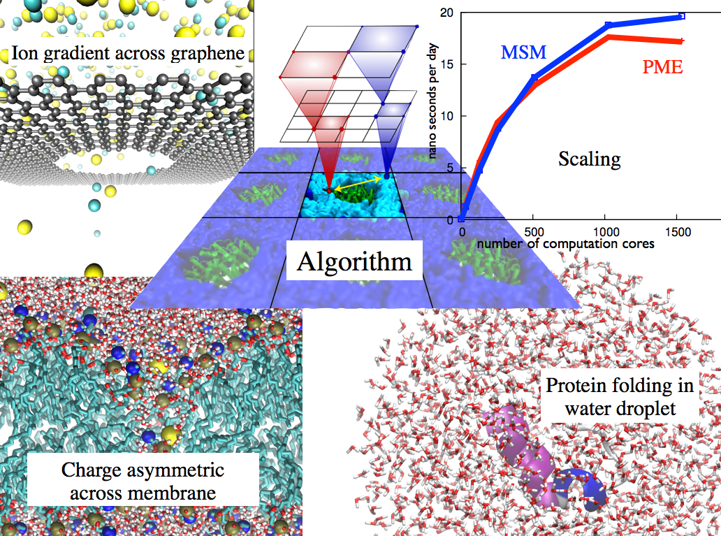
![[MSM impact summary]](msm_summary_small.jpg)
|
|
|
Figure 2 - Summary of scientific impact for MSM. (Full sized image: 1.2 MB.) |
The MSM overcomes parallel scalability issues inherent in the particle-mesh Ewald (PME) method while enabling new capabilities for simulation. PME approximates electrostatic interactions through the use of the fast Fourier transform (FFT). However, an FFT-based approximation generally requires simulations to describe infinite three-dimensional lattices, where each lattice cell is filled with a copy of the simulated system. The communication cost of calculating in parallel the two 3D FFTs required by PME outpaces the computational cost as the number of atoms and number of processors increase, due to the necessity of exchanging data between all of the processors involved in the FFT calculation. The MSM effectively replaces the non-scalable FFT communication by more densely localized convolution calculations that permit better parallel scaling and utilization of modern vector computational hardware units. Furthermore, the MSM directly supports simulations employing nonperiodic or semiperiodic boundary conditions. Examples include the semiperiodic simulation of asymmetric charge across a membrane bilayer or of an ion gradient across a graphene nanopore and the nonperiodic simulation of protein folding in a water droplet. These applications are discussed further on the main research page.
Publications
-
Publications Database Multilevel summation with B-spline interpolation for pairwise interactions in molecular dynamics simulations. David J. Hardy, Matthew A. Wolff, Jianlin Xia, Klaus Schulten, and Robert D. Skeel. Journal of Chemical Physics, 144:114112, 2016. (16 pages). -
Publications Database Multilevel summation method for electrostatic force evaluation. David J. Hardy, Zhe Wu, James C. Phillips, John E. Stone, Robert D. Skeel, and Klaus Schulten. Journal of Chemical Theory and Computation, 11:766-779, 2015. -
Publications Database Multilevel summation of electrostatic potentials using graphics processing units. David J. Hardy, John E. Stone, and Klaus Schulten. Journal of Parallel Computing, 35:164-177, 2009.
Investigators
Collaborators
Page created and maintained by David Hardy.


