Modeling Biological Processes at Hybrid Resolutions
Computational challenge of simulating biological processes
Computer simulations have become an indispensable tool for revealing the molecular mechanism of biological processes. They could provide atomistic details of the processes that are hardly observed through experimental measurements. However, since biological processes, which are normally microsecond or even millisecond long, need to be followed in computer simulations femtosecond by femtosecond, simulating such processes in every atomistic detail is computationally challenging. Despite ever-growing computing power, computer simulations cannot be used for the modeling of large biomolecular systems over time scales long enough to be of biological interest. To overcome the challenge, coarse-grained models, in which multiple atomistic sites are grouped into one site, have been developed for components of biomolecular systems, such as proteins, solvent and membrane (see Marrink's and our coarse-graining website). The models significantly reduce computational cost and, thereby, enhance the speed of simulation. However, because of inherent simplification that omits important structural details of proteins, many coarse-grained simulations of proteins rely on information from native protein structures. The coarse-grained models are limited, therefore, in their use in studies of folding, aggregation, large conformational changes of proteins, or conformational features of intrinsically disordered proteins.
Development of a hybrid model
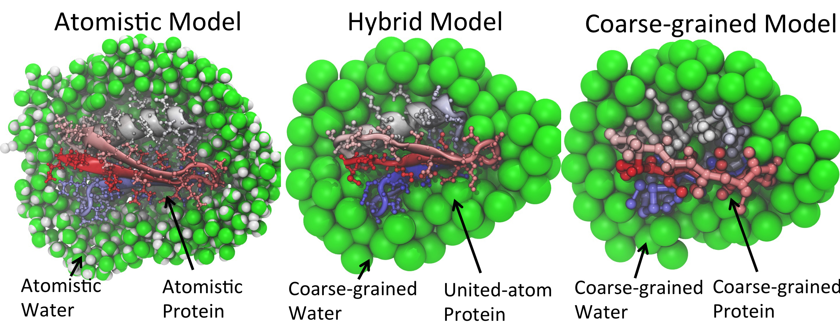
Representation of a solvated protein at different levels of details. Protein G (PDB ID: 3GB1) is chosen for the illustration.
To alleviate the reliance on native structures, several coarse-grained protein models have been parametrized to reproduce peptide folding or have been built on knowledge-based statistical potentials, achieving even in some cases predictive capabilities. Nevertheless, it may be more advantageous to combine atomistic and coarse-grained models so that protein models contain enough atomistic detail to obviate the need for information about native structures while environments such as water and membrane are still coarse-grained. By following this idea, a hybrid model with its components represented at different levels of details has been developed. In this model, most of atomistic details of proteins are maintained but all hydrogen atoms are omitted, with an exception of the ones in backbones of proteins; environments are, on the other hand, represented with residue-based coarse-grained models developed by Marrink et al. (see Marrink and also our coarse-graining website) where about every ten atoms are reduced to one site. This hybrid model was conceived on the basis of the following considerations:
(1) Interactions such as hydrogen bonding of backbones and packing of side chains are crucial for secondary and tertiary structures of proteins. For a model containing atomistic details of proteins, there is no need to use complicated functional forms to describe interactions in proteins but the simple ones, such as Lennard-Jones and Coulombic potentials, which are easier to obtain parameters for;
(2) With the simple functional forms for energetics, the model should be ready for use with mainstream computer simulation softwares, such as NAMD;
(3) Instead of building up a new coarse-grained model for environment from scratch, it would be better to begin with existing models, such as the one by Marrink et al. that has been widely used in simulations of water and membrane.
Tremendous efforts have been spent in parameterizing the hybrid model in order to make it accurate enough for computational studies of proteins. For example, conformational parameters of backbones and side chains of proteins has been calibrated with a database from Protein Data Bank; the interactions between atomistic proteins and coarse-grained environments are parametrized by reproducing experimental thermodynamic stability of a large set of organic molecules in water or across membrane. As reported recently, we have significantly improved the model for simulations of protein folding by re-parameterizing hydration of protein backbones, a critical factor for controlling the balance between unfolded and folded states of proteins.
Simulations of protein folding with the hybrid model
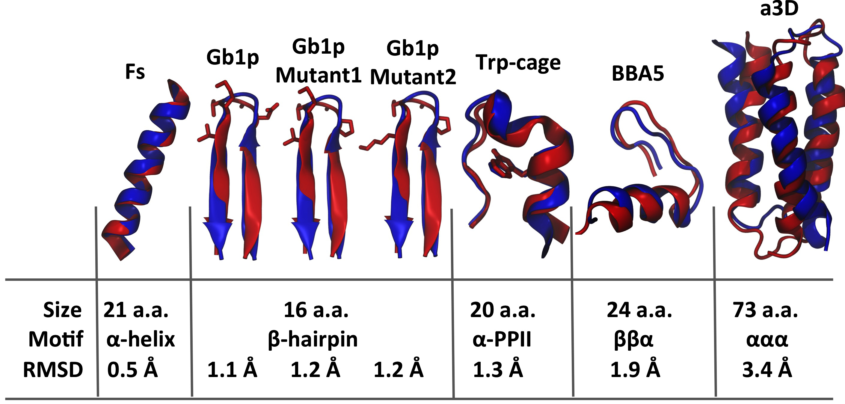
Summary of seven small proteins used for folding simulations, including their sizes, structural motifs and difference between experimental and simulated structures for each protein. The difference was measured by root mean square deviation (RMSD) of positions of backbone atoms between experimental and simulated structures. Structural superpositions between two type of structures show that experimental structures (red) were well reproduced by simulations (blue) with the hybrid model.
How proteins fold into their native structures is a fundamental but mysterious biological process. Observing such a process in computers requires that computational models are able to provide an accurate description of energetics for both proteins and their environments. In fact, protein folding has been recognized as an important opportunity for validation and improvement of computational models. To verify the hybrid model, we carried out folding simulations of a series of small proteins, as summarized in the figure on the right. These proteins have a wide spectrum of structural motifs, including α-helix (Fs), β-strand (GB1p and its mutants), α-PPII (Trp cage), ββα (BBA5), and ααα (α3D) systems, providing a robust test of whether the model is balanced among different structures. All the folding simulations, without any prior knowledge of native structures, started with random structures and ended up with structures very close to the ones seen in experiments.
Since conformational complexity of proteins grows exponentially with their size, α3D, a three-helix bundle protein that is almost twice larger than the other tested proteins, would exhibit folding events that need much longer simulations to observe. Therefore, folding of α3D in computers is considerably more challenging, which has become possible only recently by using a special-purpose machine, Anton, and at an elevated simulation temperature intended for acceleration. With help of the hybrid model, we have observed complete folding events of α3D at the physiological temperature in three independent simulations, each of them starting with entirely different random structures.
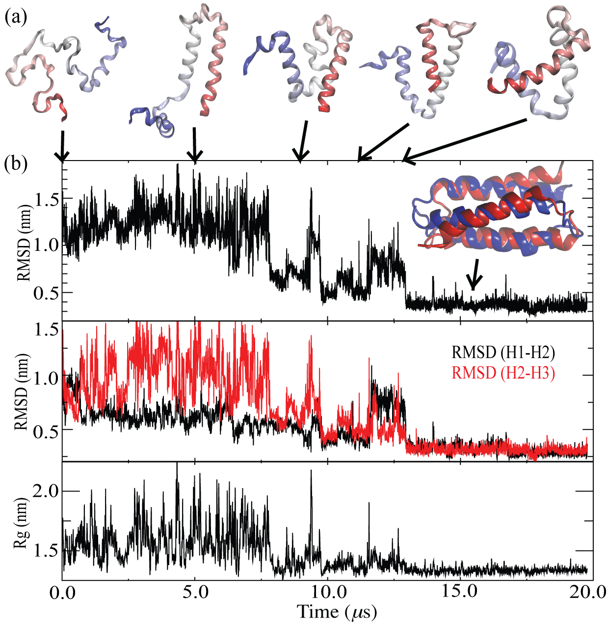
Evolutions of structures of α3D during one of the folding simulations. (a) displays structures of the protein in selected frames from the simulation. (b) show progressive changes of various structural features, including RMSD for the entire protein (top panel), RMSD for either regions H1 and H2 (black) as a whole or regions H2 and H3 (red) as a whole (middle panel), and radius of gyration of the protein (bottom panel).
Close-up inspections on these simulations help us to understand interesting features of α3D folding. For instance, what do unfolded states look like? Our simulations reveal that unfolded states of α3D are disordered and keep changing their shapes, as reflected by large fluctuations in their radius of gyration, a quantity describing overall shapes of proteins (as shown in the figure on the left). However, the unfolded states do display significant (about 25%) residual helical content. A residual helical content of 20% had also been reported for unfolded α3D in the simulations with Anton.
There are three helical regions in α3D helical bundle structures, namely, H1 (residues 1-18), H2 (residues 28-44), and H3 (residues 54-73). It is natural to wonder how these helical regions assemble into the native bundle structures. As all the simulations progress, we observed that regions H1 and H2 as a whole form native-like structures earlier than regions H2 and H3 do (as shown by the results of structural deviation calculation in the figure on the left), which means that there is a tendency for α3D to form a native helical bundle between H1 and H2 before a H2-H3 bundle could be formed. However, how the three regions actually assemble is more complicated. We have observed different pathways on which α3D reaches the native bundle structure. In two of the three simulations, folding was complete after H3 packed itself to the preformed H1-H2 bundle with correct native contacts (Movie), following the aforementioned tendency; in a third simulation emerged intermediates with native like topologies but a non-native hydrophobic core, which dwelled for microseconds [8 μs < t < 13 μs (the left figure)] but eventually transited to the folded structure (Movie). Such a scenario of multiple folding pathways is expected for α3D according to experiments.
To investigate α3D folding, we have collected in total 60-microsecond long simulations which are quite staggering in the sense of simulation length. So, how much computation did these simulations actually take? It turned out that the simulations were done just in a month only with easy-to-access computational resources, i.e., desktop computers, which are nothing compared to the super machines like Anton that may be too expensive for whoever is interested in folding simulations.
Constructing folding landscape with the hybrid model
An even more challenging task is to systematically investigate folding mechansims of proteins, which acquires thorough knowledge of free energy surfaces (FES) governing protein folding and of the associated folding mechanisms. Computational characterization of folding mechanisms and their underlying FES is a difficult task. One of the major reasons for the difficulty is that due to high dimensionality, it is complicated to determine and represent the FES and subsequently extract folding kinetics from it. In the past decade, new methods based on network analysis have been proposed to characterize the FES of folding through graphical representations of the FES. In short, FES of folding could be considered as conformational transition networks in which each node denotes a kinetic stable state while conformational transitions among the stable states are represented by links between nodes. Such a network could be analyzed, using standard graph theory, to derive many important properties of proteins regarding their folding mechanisms.
The network analysis of the folding FES usually requires unbiased folding simulations of proteins. Ideally, the simulations need to include full atomistic detail and need to sample multiple folding and unfolding events. In practice, obtaining such simulations is difficult owing to the long timescale for folding events to arise and due to the requirement of powerful computational resources needed for all-atom molecular dynamics (MD) simulations. it is still desirable to explore the FES of folding through a less expensive computational approach. One option is to replace the atomistic representation by a coarse-grained (CG) model, which groups multiple atomic ort becomes signicantly reduced. simulations with CG models are normally assisted by Go-like potentials. Several CG models that do not rely on Go-like potentials have been applied to fold unstructured proteins to their native structures, but none of them have been used to perform also a network analysis to examine the folding FES.
It would be interesting to see whether our hybrid model could be used to capture folding networks for proteins. To this end, two known fast-folding proteins have been investigated through a combination of multiple folding simulations and a subsequent network analysis of free energy surfaces. One protein studied is a helical protein, namely Trp-cage, and the other is a three-stranded β-sheet protein, namely one related to hPin WW domains. One benefitt of our model is that folding kinetics are accelerated by about two orders of magnitude in simulations with the model. Therefore, multiple folding and unfolding events have been seen in microseonds of simulations, allowing us to construct a comprehensive folding network. The network analysis revealed complicated folding landscapes for both proteins: although in both cases the native structures are the most-populated states among all the states, several non-native structures are considerably populated and clearly discernible as folding intermediates, a feature having also been seen in previous atomic simulations.
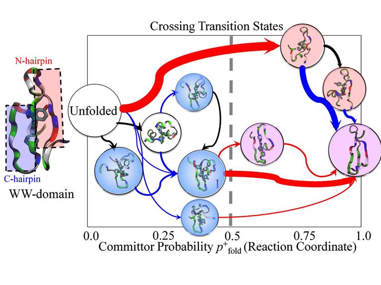
Folding network of WW domains. Shown in pink color are the states where hairpin 1 forms. Shown in blue color are the states where hairpin 2 forms. Shown in purple color are the states with both hairpins. Red and blue arrows denote conformational transitions involved with formation of hairpins 1 and 2, respectively.
The constructed folding networks helped us resolve the folding mechanisms of the proteins. For example, one question regarding folding mechanisms of WW domains, as shown in the figure on the right, is which of its two hairpins fold first. The network constructed by us revealed that hairpin 2 has 80 % of a chance to form first during the course of folding while hairpin 1 has only 20 % of a chance to happen first. Interestingly, although hairpin 1 has less chance to be the first to form, its formation is actually the rate-determining step of the overall folding process no matter which hairpin forms first. For the case where hairpin 2 forms first, its fomation is mostly completed before transition states could be reached. Thus, it cannot be the rate-determining steps. Our observation that hairpin 1 involves the rate-determining steps of the folding agrees with experiments which showed that modifications of hairpin 1 greatly changes the folding kinetics of WW domains. In summary, our hybrid model is not only useful for folding simulations, but also for the characterization of free energy surfaces and folding pathways.
Movies
pathA.mpg (11.5MB): Folding pathway via nonntaive contacts.
pathB.mpg (5.0MB): Folding pathway via packing of H3 to preformed H1-H2 bundle.
Download the model
Publications
Characterization of Folding Mechanisms of Trp-Cage and WW-Domain by Network Analysis of Simulations with a Hybrid-Resolution Model. Wei Han, and Klaus Schulten Journal of Chemical Theory and Computation, 117:13367-13377, 2013
Further optimization of a hybrid united-atom and coarse-grained force field for folding simulations: improved backbone hydration and interactions between charged side chains. Wei Han, and Klaus Schulten Journal of Chemical Theory and Computation, 8:4413-4424, 2012
Parameterization of PACE force field for membrane environment and simulation of helical peptides and helix-helix association. Cheuk-Kin, Wan, Wei Han, and Yundong Wu Journal of Chemical Theory and Computation, 8:300-313, 2012
PACE force field for protein simulations. 2. Folding simulations of peptides. Wei Han, Cheuk-Kin Wan, and Yundong Wu Journal of Chemical Theory and Computation, 6:3390-3402, 2010
PACE force field for protein simulations. 1. Full parameterization of version 1 and verification. Wei Han, Cheuk-Kin Wan, Fan Jiang, and Yundong Wu Journal of Chemical Theory and Computation, 6:3373-3389, 2010
Toward a coarse-grained protein model coupled with a coarse-grained solvent model: solvation free energies of amino acid side chains. Wei Han, Cheuk-Kin Wan, and Yundong Wu Journal of Chemical Theory and Computation, 4:1891-1901, 2008
Coarse-grained protein model coupled with a coarse-grained water model: molecular dynamics study of polyalanine-based peptides. Wei Han, and Yundong Wu Journal of Chemical Theory and Computation, 3:2146-2161, 2007
Investigators
Page created and maintained by Wei Han.