• Home

• Overview

• Publications

• Research

• Driving Biomedical Projects

• Collaborations

• Viruses

• Symbiont Bacteria

• Molecular Motors

• Neurons and Synapses

• Bioenergetic Membranes

• Nanosensors

• Ribosome

• Mechanosensing

• Protein Folding

• Integrative Modeling

• More Topics

• Software

• Outreach

Kinetic Diffusion

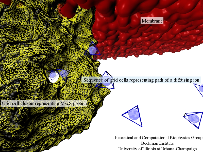
Fig. 1.Illustration of discretized model of ion diffusion (blue spheres within blue-edged cells) near a mechanosensitive channel of small conductance (yellow-edged cells) embedded in a biological membrane (red).

There are many ways of describing diffusion in a biological system. Free diffusion models based on the Green's function of the diffusion equation and random walk algorithms have been used to describe diffusion of biomolecules over the length scale of organelles and entire cells, on the order of micrometers, while highly-detailed Brownian dynamics and molecular dynamics have been used in simulations of diffusion over molecular length scales on the order of Ångstroms. Between the cellular and molecular length scales exists a middle ground where diffusion occurs over an intermediate length scale that is too large for atomistic models to be computed inexpensively and yet not large enough that the local potential and diffusivity fields can be neglected.

For example, the dynamics of ions translocating through an ion channel is affected by the diffusive approach of the ions in a large neighborhood hundreds of Ångstroms around the channel as well as the Ångstrom-scale variations in channel geometry and the potential and diffusivity fields near and within the channel. Few methods that efficiently simulate systems on these intermediate length scales and the corresponding typical diffusion time scales incorporate such detailed parameters. Driven by the challenge of simulating an ion channel on these scales, we combined the high resolution descriptive power of molecular dynamics with the efficiency of a finite-element calculation in a particle-based method to describe systems on these intermediate length and time scales.

In order to incorporate the Ångstrom-scale details of the system, we first perform a long-time molecular dynamics simulation of the channel implanted in a membrane and immersed in a large waterbox containing the diffusing particles. The potential and diffusivity fields, U(r) and D(r) respectively, are extracted by averaging over time the particle concentration and mean squared displacement per unit time. The geometry of the system is implicit in the potential field, an example of which is shown in Figure 5. The potential and diffusivity fields are input parameters of the Smoluchowski equation, which the diffusion model described below is based on.

In our diffusion model, the system is first discretized on an irregular grid that assigns higher densities of cells to regions which require a detailed description, such as the neighborhood of an ion channel, and lower densities of cells to regions that are more uniform, such as empty space far away from the channel. With a good cell distribution, this discretization scheme makes the method more computationally affordable. Diffusing particles diffuse in the system by hopping across the grid in a series of time steps. For each hop, a particle chooses the target grid cell stochastically using a transition probability calculated from the Smoluchowski equation, given below:

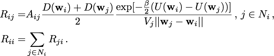
The Smoluchowski equation describes the time evolution of probability distribution given an initial distribution, a potential field U(r) and a diffusivity field D(r). The equation is discretized by integrating over the cell currently occupied by the particle. The result of this integration is a set of probability flow rates R_ij into the current cell I_i from its nearest neighbors I_j, where j is an element of the set N_i of indices labelling the nearest neighbors of I_i. These probability flow rates depend on the potentials and diffusivities assigned by the pre-obtained fields to the respective cells, as well as the geometric properties of the cells, as described in Figure 2a. For each i, R_ii, which is the retention rate of particles within I_i, is the negative of the sum over j of R_ji, so as to conserve the particle number.

Setting then R_ij = 0 for j that are not in N_i, the kinetics of a particle moving from one cell to a nearest neighbor can be described by the master equation

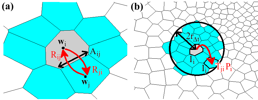
Fig. 2. Schematic of the diffusion model. (a) Probability flow rates between I_i (pink) and nearest neighbors I_j (blue) specified in the master equation depend on the volume V_i of I_i, the interfacial area A_ij between I_i and I_j, and the distance between the cell centers w_i and w_j. (b) Transition probability T_ji from I_i to I_j for a particle initially in I_i after time Δt. The transition probability is obtained by integrating the master equation restricted to a neighborhood within a radius 2r_Δt of I_i.

The next step is to calculate, given that the particle is initially in I_i, the probability distribution over the grid after one time step Δt has elapsed. Such a calculation can become very expensive on large grids. Fortunately, it can be approximated heuristically that the particle is effectively confined within a certain neighborhood, of size dependent on the time step and characterized by length r_Δt, of its initial position. Hence, one can restrict the master equation (by including only the relevant matrix and vector elements) to the cells within this neighborhood. For each i, R_ii must be re-calculated to preserve particle conservation. The restricted master equation is then integrated over time Δt, assuming that the particle is initially in I_i, to give T_ji, the probability of transition from I_i to I_j, where I_j is a cell within the neighborhood of I_i but not necessarily a nearest neighbor. Figure 2b illustrates a possible transition in one time step Δt within the restricted neighborhood. Finally, setting T_ij = 0 for all j not in the neighborhood of I_i, we can write for T_ij an analogy to the master equation in R_ij:

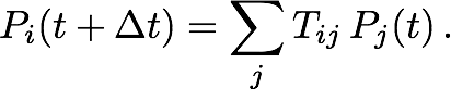
We tested our diffusion model by using it to describe simple systems, consisting of particles diffusing between two concentric spheres. Reflective boundary conditions were imposed on the outer sphere and absorptive boundary conditions on the inner sphere. The simulations were run with both a flat potential as well as a harmonic potential centered on the centers of the spheres. For different parameter values, the number of surviving particles, for which the analytic behaviors are known, were tracked over time and compared to the analytic behaviors. Figure 2 shows that for different values of time step size (2a) and grid densities (2b), the model agreed well with the analytic predictions for free diffusion. Figure 3 shows that the model holds up well after the addition of a harmonic potential, again for different values of time step size (3a) and grid densities (3b).

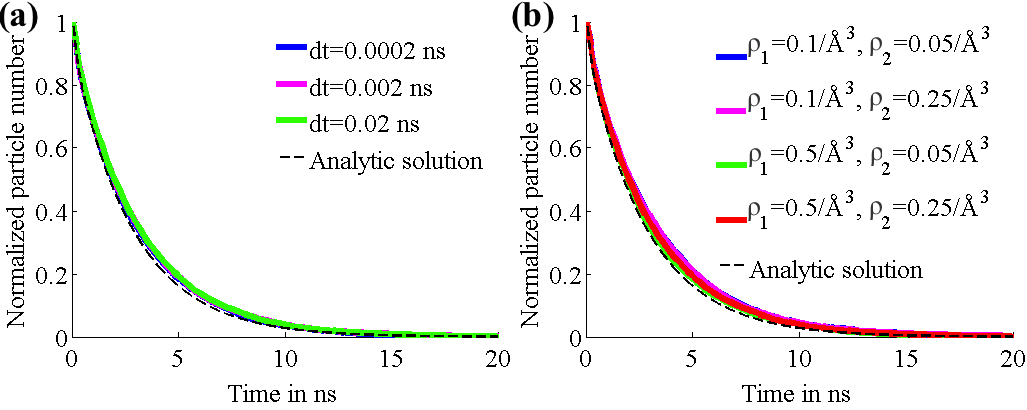
Fig. 3. Number of surviving particles for system with flat potential. Graphs for each case are superimposed and thus obscure each other.

Fig. 4. Number of surviving particles for system with harmonic potential. Graphs for each case are superimposed and thus obscure each other.

We also simulated the diffusion of K⁺ and glutamate (Glu^-) ions through the mechanosensitive channel of small conductance (MscS) and measured conduction rates, with the same bias potentials used in BioMOCA simulations of the MscS in an earlier study. Our results are in agreement with the previous study in the case of K⁺. In the case of the anion, since the previous study used Cl^- as opposed to Glu^-, there are significant differences in the conductance rates. Careful consideration of the reasons for these differences pointed to steric factors (Glu^- is much bigger than Cl^-) and more importantly, the lack of inter-particle interactions in our model. Inter-particle interactions will thus be the next step in the development of our model.

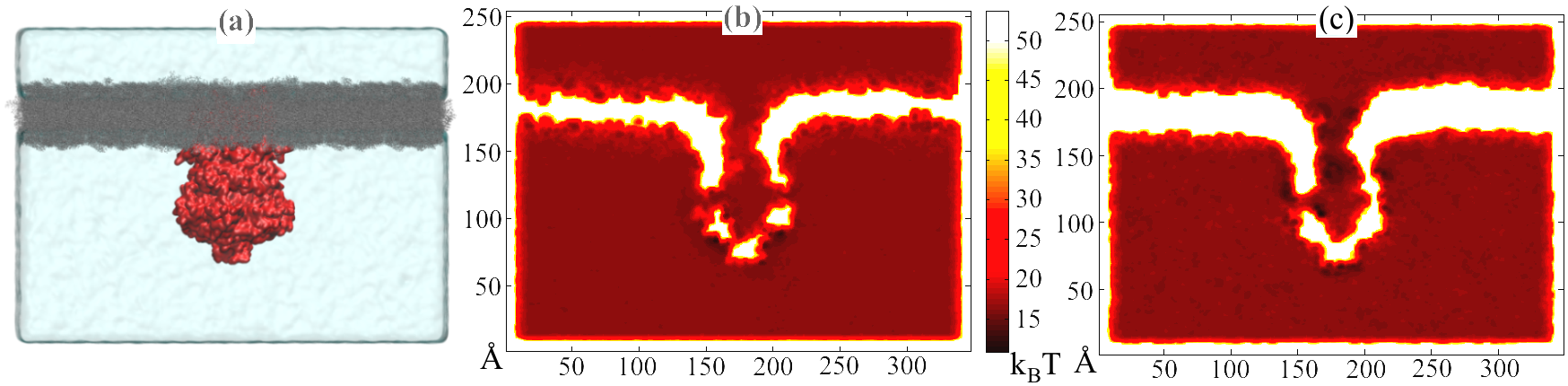
Fig. 5. (a) System used in molecular dynamics simulation. MscS (red) is embedded in a lipid bilayer (grey) and solvated in a waterbox. Also shown are potential maps of the same system for ions (b) K⁺ and (c) Glu^-.