Free Energy of Conformational Change Calculations

Next: Adaptive Biasing Force Calculations Up: Additional Simulation Parameters Previous: Applied Forces and Analysis Contents Index

Subsections

Free Energy of Conformational Change Calculations

NAMD incorporates methods for performing free energy of conformational change perturbation calculations. The system is efficient if only a few coordinates, either of individual atoms or centers of mass of groups of atoms, are needed. The following configuration parameters are used to enable free energy perturbation:

freeEnergy is free energy perturbation active?
Acceptable Values: on or off
Default Value: off
Description: Specifies whether or not free energy perturbation is active. If it is set to off, then no free energy perturbation is performed. If it is set to on, then the free energy perturbation calculation specified in freeEnergyConfig parameters is executed.
freeEnergyConfig free energy perturbation script
Acceptable Values: file or {script}
Description: Must contain either the name of a free energy perturbation script file or the script itself between { and } (may include multiple lines). This parameter may occur multiple times and scripts will be executed in order of appearance. The format of the free energy perturbation script is described below.

The following sections describe the format of the free energy perturbation script.

User-Supplied Conformational Restraints

These restraints extend the scope of the available restraints beyond that provided by the harmonic position restraints. Each restraint is imposed with a potential energy term, whose form depends on the type of the restraint.

Fixed Restraints

Position restraint (1 atom): force constant $K_{f}$ , and reference position $\overrightarrow{r_{ref}}$

$\qquad \qquad \qquad \qquad E=\left( K_{f}/2\right) \left( \left\vert \overrightarrow{r_{i}}-\overrightarrow{r_{ref}}\right\vert \right) ^{2}$

Stretch restraint (2 atoms): force constant $K_{f}$ , and reference distance $d_{ref}$

$\qquad \qquad \qquad \qquad E=\left( K_{f}/2\right) \left( d_{i}-d_{ref}\right) ^{2}$

Bend restraint (3 atoms): force constant $K_{f}$ , and reference angle $\theta _{ref}$

$\qquad \qquad \qquad \qquad E=\left( K_{f}/2\right) \left( \theta _{i}-\theta _{ref}\right) ^{2}$

Torsion restraint (4 atoms): energy barrier $E_{0}$ , and reference angle $\chi _{ref}$

$\qquad \qquad \qquad \qquad E=\left( E_{0}/2\right) \left\{ 1-\cos \left( \chi _{i}-\chi _{ref}\right) \right\}$

Forcing restraints

Position restraint (1 atom): force constant $K_{f}$ , and two reference positions $\overrightarrow{r_{0}}$ and $\overrightarrow{r_{1}}$

$\qquad \qquad \qquad \qquad E=\left( K_{f}/2\right) \left( \left\vert \overrightarrow{r_{i}}-\overrightarrow{r_{ref}}\right\vert \right) ^{2}$

$\qquad \qquad \qquad \qquad \overrightarrow{r_{ref}}$ $=\lambda \overrightarrow{r_{1}}+\left( 1-\lambda \right)$ $\overrightarrow{r_{0}}$

Stretch restraint (2 atoms): force constant $K_{f}$ , and two reference distances $d_{0}$ and $d_{1}$

$\qquad \qquad \qquad \qquad E=\left( K_{f}/2\right) \left( d_{i}-d_{ref}\right) ^{2}$

$\qquad \qquad \qquad \qquad d_{ref}=d_{1}+\left( 1-\lambda \right) d_{0}$

Bend restraint (3 atoms): force constant $K_{f}$ , and two reference angles $\theta _{0}$ and $\theta _{1}$

$\qquad \qquad \qquad \qquad E=\left( K_{f}/2\right) \left( \theta _{i}-\theta _{ref}\right) ^{2}$

$\qquad \qquad \qquad \qquad \theta _{ref}=\lambda \theta _{1}+\left( 1-\lambda \right) \theta _{0}$

Torsion restraint (4 atoms): energy barrier E $_{0}$ , and two reference angles $\chi _{0}$ and $\chi _{1}$

$\qquad \qquad \qquad \qquad E=\left( E_{0}/2\right) \left\{ 1-\cos \left( \chi _{i}-\chi _{ref}\right) \right\}$

$\qquad \qquad \qquad \qquad \chi _{ref}=\lambda \chi _{1}+\left( 1-\lambda \right) \chi _{0}$

The forcing restraints depend on the coupling parameter, $\lambda$ , specified in a conformational forcing calculation. For example, the restraint distance, $d_{ref}$ , depends on $\lambda$ , and as $\lambda$ changes two atoms or centers-of-mass are forced closer together or further apart. In this case $K_{f}$ = $K_{f,0}$ , the value supplied at input.

Alternatively, the value of $K_{f}$ may depend upon the coupling parameter $\lambda$ according to:

$K_{f}$ = $K_{f,0} \lambda$

Bounds

Position bound (1 atom): Force constant $K_{f}$ , reference position $\overrightarrow{r_{ref}}$ ,

and upper or lower reference distance, $d_{ref}$

Upper bound:

$\qquad \qquad \qquad \qquad E=\left( K_{f}/2\right) \left( d_{i}-d_{ref}\right) ^{2}$ for $d_{i}>d_{ref}$ , else .

Lower bound:

$\qquad \qquad \qquad \qquad E=\left( K_{f}/2\right) \left( d_{i}-d_{ref}\right) ^{2}$ for $d_{i}$ $d_{ref}$ , else .

$\qquad \qquad \qquad \qquad d_{i}^{2}=\left( \left\vert \overrightarrow{r_{i}}- \overrightarrow{r_{ref}}\right\vert \right) ^{2}\medskip\medskip$

Distance bound (2 atoms): Force constant $K_{f}$ ,

and upper or lower reference distance, $d_{ref}$

Upper bound:

$\qquad \qquad \qquad \qquad E=\left( K_{f}/2\right) \left( d_{ij}-d_{ref}\right) ^{2}$ for $d_{ij}>d_{ref}$ , else .

Lower bound:

$\qquad \qquad \qquad \qquad E=\left( K_{f}/2\right) \left( d_{ij}-d_{ref}\right) ^{2}$ for $d_{ij}<d_{ref}$ , else .

Angle bound (3 atoms): Force constant $K_{f}$ ,

and upper or lower reference angle, $\theta _{ref}$

Upper bound:

$\qquad \qquad \qquad \qquad E=\left( K_{f}/2\right) \left( \theta -\theta _{ref}\right) ^{2}$ for $\theta >\theta _{ref},$ else .

Lower bound:

$\qquad \qquad \qquad \qquad E=\left( K_{f}/2\right) \left( \theta -\theta _{ref}\right) ^{2}$ for $\theta <\theta _{ref},$ else $E=0.\medskip\medskip \medskip$

Torsion bound (4 atoms): An upper and lower bound must be provided together.

Energy gap $E_{0}$ , lower AND upper reference angles, $\chi _{1}$ and $\chi _{2}$ ,

and angle interval, $\Delta \chi .$

$\chi _{1}$ $<\chi$ $<\chi _{2}$ :

$\left( \chi _{1}-\Delta \chi \right)$ $<\chi$ $<\chi _{1}$ : $E=\left( G/2\right) \left\{ 1-\cos \left( \chi -\chi _{1}\right) \right\}$

$\chi _{2}$ $<\chi$ $\left( \chi _{2}+\Delta \chi \right)$ : $E=\left( G/2\right) \left\{ 1-\cos \left( \chi -\chi _{2}\right) \right\}$

$\left( \chi _{2}+\Delta \chi \right) ~$ $<\chi$ $\left( \chi _{1}-\Delta \chi +2\pi \right)$ :

$\qquad \qquad G=E_{0}/\left\{ 1-\cos \left( \Delta \chi \right) \right\} \bigskip$

Bounds may be used in pairs, to set a lower and upper bound. Torsional bounds always are defined in pairs.

Free Energy Calculations

Conformational forcing / Potential of mean force

In conformational forcing calculations, structural parameters such as atomic positions, inter-atomic distances, and dihedral angles are forced to change by application of changing restraint potentials. For example, the distance between two atoms can be restrained by a potential to a mean distance that is varied during the calculation. The free energy change (or potential of mean force, pmf) for the process can be estimated during the simulation.

The potential is made to depend on a coupling parameter, $\lambda$ , whose value changes during the simulation. In potential of mean force calculations, the reference value of the restraint potential depends on $\lambda$ . Alternately, the force constant for the restraint potential may change in proportion to the coupling parameter. Such a calculation gives the value of a restraint free energy, i.e., the free energy change of the syste

m due to imposition of the restraint potential.

Methods for computing the free energy

With conformational forcing (or with molecular transformation calculations) one obtains a free energy difference for a process that is forced on the system by changing the potential energy function that determines the dynamics of the system. One always makes the changing potential depend on a coupling parameter, $\lambda$ . By convention, $\lambda$ can have values only in the range from to , and a value of $\lambda =0$ corresponds to one defined state and a value of $\lambda =1$ corresponds to the other defined state. Intermediate values of $\lambda$ correspond to intermediate states; in the case of conformational forcing calculations these intermediate states are physically realizable, but in the case of molecular transformation calculations they are not.

The value of $\lambda$ is changed during the simulation. In the first method provided here, the change in $\lambda$ is stepwise, while in the second method it is virtually continuous.

Multi-configurational thermodynamic integration (MCTI).

In MCTI one accumulates $\,\left\langle \partial U/\partial \lambda \right\rangle$ at several values of $\lambda$ , and from these averages estimates the integral

$-\Delta A=\int \,\left\langle \partial U/ \partial \lambda \right\rangle d\lambda$

With this method, the precision of each $\left\langle \partial U/\partial \lambda \right\rangle$ can be estimated from the fluctuations of the time series of $\partial U/\partial \lambda$ .

Slow growth.

In slow growth, $\lambda$ is incremented by $\delta \lambda =\pm 1/N_{step}$ after each dynamics integration time-step, and the pmf is estimated as

$-\Delta A=\Sigma$ $\left( \partial U/\partial \lambda \right)$ $\delta \lambda$

Typically, slow growth is done in cycles of: equilibration at $\lambda =0$ , change to $\lambda =1$ , equilibration at $\lambda =1$ , change to $\lambda =0$ . It is usual to estimate the precision of slow growth simulations from the results of successive cycles.

Options for Conformational Restraints

User-supplied restraint and bounds specifications

urestraint $\{$

n * (restraint or bound specification) // see below

$\}\medskip$

Restraint Specifications (not coupled to pmf calculations)

posi ATOM kf = KF ref = (X Y Z)

dist 2 x ATOM kf = KF ref = D

angle 3 x ATOM kf = KF ref = A

dihe 4 x ATOM barr = B ref = A

Bound Specifications (not coupled to pmf calculations)

posi bound ATOM kf = KF [low = (X Y Z D) or hi = (X Y Z D)]

dist bound 2 x ATOM kf = KF [low = D or hi = D]

angle bound 3 x ATOM kf = KF [low = A or hi = A]

dihe bound 4 x ATOM gap = E low = A0 hi = A1 delta = A2

Forcing Restraint Specifications (coupled to pmf calculations)

posi pmf ATOM kf=KF low = (X0 Y0 Z0)    hi = (X1 Y1 Z1)

dist pmf 2 x ATOM kf=KF low = D0    hi = D1

angle pmf 3 x ATOM kf=KF low = A0    hi = A1

dihe pmf 4 x ATOM barr=B low = A0    hi = A1

Units

Input item Units

E, B kcal/mol

X, Y, Z, D

A degrees

$K_{f}$ kcal/(mol $^{2}$ ) or kcal/(mol rad $^{2}$ )

Options for ATOM Specification

The designation ATOM, above, stands for one of the following forms:

A single atom

(segname, resnum, atomname)

Example: (insulin, 10, ca)

All atoms of a single residue

(segname, resnum)

Example: (insulin, 10)

A list of atoms

group $\{$ (segname, resnum, atomname), (segname, resnum, atomname), $\ldots$ $\}$

Example: group $\{$ (insulin, 10, ca), (insulin, 10, cb), (insulin, 11, cg) $\}\medskip$

All atoms in a list of residues

group $\{$ (segname, resnum), (segname, resnum), $\ldots$ $\}$

Example: group $\{$ (insulin, 10), (insulin, 12), (insulin, 14) $\}\medskip$

All atoms in a range of residues

group $\{$ (segname, resnum) to (segname, resnum) $\}$

Example: group $\{$ (insulin, 10) to (insulin, 12) $\}\medskip$

One or more atomnames in a list of residues

group $\{$ atomname: (segname, resnum), (segname, resnum), $\ldots$ $\}$

group $\{$ (atomname, atomname, $\ldots$ ): (segname, resnum), (segname, resnum), $\ldots$ $\}$

Examples: group $\{$ ca: (insulin, 10), (insulin, 12), (insulin, 14) $\}$

group $\{$ (ca, cb, cg): (insulin, 10), (insulin, 12), (insulin, 14) $\}$

group $\{$ (ca, cb): (insulin, 10), (insulin, 12) cg: (insulin, 11), (insulin, 12) $\}\smallskip$

Note: Within a group, atomname is in effect until a new atomname is used, or the keyword all is used. atomname will not carry over from group to group. This note applies to the paragraph below.

One or more atomnames in a range of residues

group $\{$ atomname: (segname, resnum) to (segname, resnum) $\}$

group $\{$ (atomname, atomname, $\ldots$ ): (segname, resnum) to (segname, resnum) $\}$

Examples: group $\{$ ca: (insulin, 10) to (insulin, 14) $\}$

group $\{$ (ca, cb, cg): (insulin, 10) to (insulin, 12) $\}$

group $\{$ (ca, cb): (insulin, 10) to (insulin, 12) all: (insulin, 13) $\}$

Options for Potential of Mean Force Calculation

The pmf and mcti blocks, below, are used to simultaneously control all forcing restraints specified in urestraint above. These blocks are performed consecutively, in the order they appear in the config file. The pmf block is used to either a) smoothly vary $\lambda$ from 0 $\rightarrow$ 1 or 1 $\rightarrow$ 0, or b) set lambda. The mcti block is used to vary $\lambda$ from 0 $\rightarrow$ 1 or 1 $\rightarrow$ 0 in steps, so that $\lambda$ is fixed while $dU/d\lambda$ is accumulated.

Lamba control for slow growth

pmf $\{$

task = [up, down, stop, grow, fade, or nogrow]

time = T [fs, ps, or ns] (default = ps)

lambda = Y (value of $\lambda$ ; only needed for stop and nogrow)

lambdat = Z (value of $\lambda _{t}$ ; only needed for grow, fade, and nogrow) (default = 0)

print = P [fs, ps, or ns] or noprint (default = ps)

$\}\medskip$

up, down, stop: $\lambda$ is applied to the reference values.

grow, fade, nogrow: $\,\lambda$ is applied to $K_{f}$ . A fixed value, $\lambda _{t}$ , is used to determine the ref. values.

up, grow: $\lambda$ changes from 0 $\rightarrow$ 1. (no value of $\,\lambda$ is required)

down, fade: $\lambda$ changes from 1 $\rightarrow$ 0. (no value of $\,\lambda$ is required)

stop, nogrow: dU/d $\lambda$ is accumulated (for single point MCTI)

Lambda control for automated MCTI

mcti $\{$

task = [stepup, stepdown, stepgrow, or stepfade]

equiltime = T1 [fs, ps, or ns] (default = ps)

accumtime = T2 [fs, ps, or ns] (default = ps)

numsteps = N

lambdat = Z (value of $\lambda _{t}$ ; only needed for stepgrow, and stepfade) (default = 0)

print = P [fs, ps, or ns] or noprint (default = ps)

$\}\medskip$

stepup, stepdown: $\lambda$ is applied to the reference values.

stepgrow, stepfade: $\lambda$ is applied to $K_{f}$ . A fixed value, $\lambda _{t}$ , is used to determine the ref. values.

stepup, stepgrow: $\lambda$ changes from 0 $\rightarrow$ 1. (no value of $\lambda$ is required)

stepdown, stepfade: $\lambda$ changes from 1 $\rightarrow$ 0. (no value of $\lambda$ is required)

For each task, $\lambda$ changes in steps of (1.0/N) from 0 $\rightarrow$ 1 or 1 $\rightarrow$ 0. At each step, no data is accumulated for the initial period T1, then dU/d $\lambda$ is accumulated for T2. Therefore, the total duration of an mcti block is (T1+T2) x N.

Examples

Fixed restraints

// 1. restrain the position of the ca atom of residue 0.

// 2. restrain the distance between the ca's of residues 0 and 10 to 5.2Å

// 3. restrain the angle between the ca's of residues 0-10-20 to 90 $^{o}$ .

// 4. restrain the dihedral angle between the ca's of residues 0-10-20-30 to 180 $^{o}$ .

// 5. restrain the angle between the centers-of-mass of residues 0-10-20 to 90 $^{o}$ .

urestraint $\{$

posi (insulin, 0, ca) kf=20 ref=(10, 11, 11)

dist (insulin, 0, ca) (insulin, 10, ca) kf=20 ref=5.2

angle (insulin, 0, ca) (insulin, 10, ca) (insulin, 20, ca) kf=20 ref=90

dihe (insulin, 0, ca) (insulin, 10, ca) (insulin, 20, ca) (insulin, 30, ca) barr=20 ref=180

angle (insulin, 0) (insulin, 10) (insulin, 20) kf=20 ref=90

$\}\bigskip$

// 1. restrain the center of mass of three atoms of residue 0.

// 2. restrain the distance between (the COM of 3 atoms of residue 0) to (the COM of 3 atoms of residue 10).

// 3. restrain the dihedral angle of (10,11,12)-(15,16,17,18)-(20,22)-(30,31,32,34,35) to 90 $^{o}$

// ( (ca of 10 to 12), (ca, cb, cg of 15 to 18), (all atoms of 20 and 22), (ca of 30, 31, 32, 34, all atoms of 35) ).

urestraint $\{$

posi group $\{$ (insulin, 0, ca), (insulin, 0, cb), (insulin, 0, cg) $\}$ kf=20 ref=(10, 11, 11)

dist group $\{$ (insulin, 0, ca), (insulin, 0, cb), (insulin, 0, cg) $\}$

group $\{$ (insulin, 10, ca), (insulin, 10, cb), (insulin, 10, cg) $\}$ kf=20 ref=6.2

dihe group $\{$ ca: (insulin, 10) to (insulin, 12) $\}$

group $\{$ (ca, cb, cg): (insulin, 15) to (insulin, 18) $\}$

group $\{$ (insulin, 20), (insulin, 22) $\}$

group $\{$ ca: (insulin, 30) to (insulin, 32), (insulin, 34), all: (insulin, 35) $\}$ barr=20 ref=90

$\}$

Bound specifications

// 1. impose an upper bound if an atom's position strays too far from a reference position.

// (add an energy term if the atom is more than 10Å from (2.0, 2.0, 2.0) ).

// 2&3. impose lower and upper bounds on the distance between the ca's of residues 5 and 15.

// (if the separation is less than 5.0Å or greater than 12.0Å add an energy term).

// 4. impose a lower bound on the angle between the centers-of-mass of residues 3-6-9.

// (if the angle goes lower than 90 $^{o}$ apply a restraining potential).

urestraint $\{$

posi bound (insulin, 3, cb) kf=20 hi = (2.0, 2.0, 2.0, 10.0)

dist bound (insulin, 5, ca) (insulin, 15, ca) kf=20 low = 5.0

dist bound (insulin, 5, ca) (insulin, 15, ca) kf=20 hi = 12.0

angle bound (insulin, 3) (insulin, 6) (insulin, 9) kf=20 low=90.0

$\}\bigskip$

// torsional bounds are defined as pairs. this example specifies upper and lower bounds on the

// dihedral angle, $\chi$ , separating the planes of the 1-2-3 residues and the 2-3-4 residues.

// The energy is 0 for: -90 $^{o}$ < $\chi$ < 120 $^{o}$

// The energy is 20 kcal/mol for: 130 $^{o}$ < $\chi$ < 260 $^{o}$

// Energy rises from 0 $\rightarrow$ 20 kcal/mol as $\chi$ increases from 120 $^{o}\rightarrow$ 130 $^{o}$ , and decreases from -90 $^{o}\rightarrow$ -100 $^{o}$ .

urestraint $\{$

dihe bound (insulin 1) (insulin 2) (insulin 3) (insulin 4) gap=20 low=-90 hi=120 delta=10

$\}$

Forcing restraints

// a forcing restraint will be imposed on the distance between the centers-of-mass of residues (10 to 15) and

// residues (30 to 35). low=20.0, hi=10.0, indicates that the reference distance is 20.0at $\lambda$ =0, and 10.0at $\lambda$ =1.

urestraint $\{$

dist pmf group $\{$ (insulin, 10) to (insulin, 15) $\}$

group $\{$ (insulin, 30) to (insulin, 35) $\}$ kf=20, low=20.0, hi=10.0

$\}\medskip$

// 1. during the initial 10 ps, increase the strength of the forcing restraint to full strength: 0 $\rightarrow$ 20 kcal/(mol $^{2}$ )

// 2. next, apply a force to slowly close the distance from 20 to 10 ( $\lambda$ changes from 0 $\rightarrow$ 1)

// 3. accumulate dU/d $\lambda$ for another 10 ps. ( stays fixed at 1)

// 4. force the distance back to its initial value of 20 ( changes from 1 $\rightarrow$ 0)

pmf $\{$

task = grow

time = 10 ps

print = 1 ps

$\}$

pmf $\{$

task = up

time = 100 ps

$\}$

pmf $\{$

task = stop

time = 10 ps

$\}$

pmf $\{$

task = down

time = 100 ps

$\}\medskip$

// 1. force the distance to close from 20 to 10 in 5 steps. ( $\lambda$ changes from 0 $\rightarrow$ 1: 0.2, 0.4, 0.6, 0.8, 1.0)

// at each step equilibrate for 10 ps, then collect dU/d $\lambda$ for another 10 ps.

// ref = 18, 16, 14, 12, 10 , duration = (10 + 10) x 5 = 100 ps.

// 2. reverse the step above ( $\lambda$ changes from 1 $\rightarrow$ 0: 0.8, 0.6, 0.4, 0.2, 0.0)

mcti $\{$

task = stepup

equiltime = 10 ps

accumtime = 10 ps

numsteps = 5

print = 1 ps

$\}$

mcti $\{$

task = stepdown

$\}$

Appendix

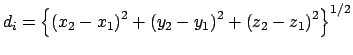
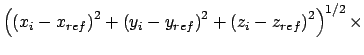
Gradient for position restraint

$E=\left( K_{f}/2\right) \left( \left\vert \overrightarrow{r_{i}}- \overrightarrow{r_{ref}}\right\vert \right) ^{2}$

$E=\left( K_{f}/2\right) \left\{ \left( x_{i}-x_{ref}\right) ^{2}+\left( y_{i}-y_{ref}\right) ^{2}+\left( z_{i}-z_{ref}\right) ^{2}\right\}$

$\nabla (E)=K_{f}\left\{ \left( x_{i}-x_{ref}\right) \overrightarrow{i} +\left( ... ...ht) \overrightarrow{j}+\left( z_{i}-z_{ref}\right) \overrightarrow{k}\right\}$

Gradient for stretch restraint

$E=\left( K_{f}/2\right) \left( d_{i}-d_{ref}\right) ^{2}$

$d_{i}=\left\{ \left( x_{2}-x_{1}\right) ^{2}+\left( y_{2}-y_{1}\right) ^{2}+\left( z_{2}-z_{1}\right) ^{2}\right\} ^{1/2}$

$\nabla (E)=K_{f}\left( d_{i}-d_{ref}\right) \cdot \nabla (di)\medskip$

for atom 2 moving, and atom 1 fixed

$\nabla (d_{i})=1/2\left\{ \left( x_{2}-x_{1}\right) ^{2}+\left( y_{2}-y_{1}\rig... ...-x_{1}\right) +2\left( y_{2}-y_{1}\right) +2\left( z_{2}-z_{1}\right) \right\}$

$\nabla (d_{i})=\left\{ \left( x_{2}-x_{1}\right) \overrightarrow{i}+\left( y_{2... ...\overrightarrow{j}+\left( z_{2}-z_{1}\right) \overrightarrow{k}\right\} /d_{i}$

$\nabla (E)=K_{f}\left\{ \left( d_{i}-d_{ref}\right) /d_{i}\right\} \left\{ \lef... ...ight) \overrightarrow{j}+\left( z_{2}-z_{1}\right) \overrightarrow{k}\right\}$

Gradient for bend restraint

$E=\left( K_{f}/2\right) \left( \theta _{i}-\theta _{ref}\right) ^{2}$

Atoms at positions A-B-C

distances: (A to B) = c; (A to C) = b; (B to C) = a;

$\theta _{i}=\cos ^{-1}(u)=\cos ^{-1}\left\{ \left( a^{2}+c^{2}-b^{2}\right) /\left( 2ac\right) \right\}$

$\nabla (E)=K_{f}\left( \theta _{i}-\theta _{ref}\right) \cdot \nabla (\theta _{i})$

$\nabla (\theta _{i})=\frac{-1}{\sqrt{1-u^{2}}}\cdot \nabla (u)\medskip$

for atom A moving, atoms B & C fixed (distances b and c change)

$\nabla (u)=\left\{ -b/\left( ac\right) \right\} \cdot \nabla (b)+\left\{ -a/\le... ...ght) +1/\left( 2a\right) +b^{2}/\left( 2ac^{2}\right) \right\} \cdot \nabla (c)$

$\nabla (b)=\left\{ \left( x_{A}-x_{C}\right) \overrightarrow{i}+\left( y_{A}-y_... ...ht) \overrightarrow{j}+\left( z_{A}-z_{C}\right) \overrightarrow{k}\right\} /b$

$\nabla (c)=\left\{ \left( x_{A}-x_{B}\right) \overrightarrow{i}+\left( y_{A}-y_... ...rightarrow{j}+\left( z_{A}-z_{B}\right) \overrightarrow{k}\right\} /c\medskip$

for atom B moving, atoms A & C fixed (distances a and c change)

$\nabla (u)=\left\{ 1/(2c)+-c/(2a^{2})+b^{2}/(2a^{2}c)\right\} \cdot \nabla (a)+... ...ft( 2c^{2}\right) +1/(2a)+b^{2}/\left( 2ac^{2}\right) \right\} \cdot \nabla (c)$

$\nabla (a)=\left\{ (x_{B}-x_{C})\overrightarrow{i}+(y_{B}-y_{C}) \overrightarrow{j}+(z_{B}-z_{C})\overrightarrow{k}\right\} /a$

$\nabla (c)=\left\{ (x_{B}-x_{A})\overrightarrow{i}+(y_{B}-y_{A}) \overrightarrow{j}+(z_{B}-z_{A})\overrightarrow{k}\right\} /c\medskip$

for atom C moving, atoms A & B fixed (distances a and b change)

$\nabla (u)=\left\{ -b/\left( ac\right) \right\} \cdot \nabla (b)+\left\{ -c/\left( 2a^{2}\right) +1/(2c)+b^{2}/\left( 2ac^{2}\right) \right\} \cdot \nabla (a)$

$\nabla (b)=\left\{ (x_{C}-x_{A})\overrightarrow{i}+(y_{C}-y_{A}) \overrightarrow{j}+(z_{C}-z_{A})\overrightarrow{k}\right\} /b$

$\nabla (a)=\left\{ (x_{C}-x_{B})\overrightarrow{i}+(y_{C}-y_{B}) \overrightarrow{j}+(z_{C}-z_{B})\overrightarrow{k}\right\} /a$

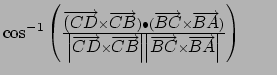
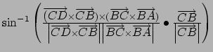
Gradient for dihedral angle restraint

$E=(E_{0}/2)\left\{ 1-\cos \left( \chi _{i}-\chi _{ref}\right) \right\}$

Atoms at positions A-B-C-D

$\chi _{i}=\cos ^{-1}(u)=$ $\cos ^{-1}\left( \frac{\overrightarrow{(CD} \times \overrightarrow{CB})\bullet ... ...\vert \overrightarrow{BC}\times \overrightarrow{BA}\right\vert }\right) \qquad$ AND

$\chi _{i}=\sin ^{-1}(v)=$ $\sin ^{-1}\left( \frac{\overrightarrow{(CD} \times \overrightarrow{CB})\times (... ...\frac{ \overrightarrow{CB}}{\left\vert \overrightarrow{CB}\right\vert }\right)$

$\nabla (E)=(E_{0}/2)\left\{ \sin \left( \chi _{i}-\chi _{ref}\right) \right\} \cdot \nabla (\chi _{i})$

$\nabla (\chi _{i})=\frac{-1}{\sqrt{1-u^{2}}}\cdot \nabla (u)\smallskip \medskip$

$\overrightarrow{CD}\times \overrightarrow{CB}$ $((y_{D}-y_{C})(z_{B}-z_{C})-(z_{D}-z_{C})(y_{B}-y_{C}))\overrightarrow{i}+$

$((z_{D}-z_{C})(x_{B}-x_{C})-(x_{D}-x_{C})(z_{B}-z_{C}))\overrightarrow{j}+$

$((x_{D}-x_{C})(y_{B}-y_{C})-(y_{D}-y_{C})(x_{B}-x_{C}))\overrightarrow{k}$

$p_{1}\overrightarrow{i}+p_{2}\overrightarrow{j} +p_{3}\overrightarrow{k}$

$\overrightarrow{BC}\times \overrightarrow{BA}=$ $((y_{C}-y_{B})(z_{A}-z_{B})-(z_{C}-z_{B})(y_{A}-y_{B}))\overrightarrow{i}+$

$((z_{C}-z_{B})(x_{A}-x_{B})-(x_{C}-x_{B})(z_{A}-z_{B}))\overrightarrow{j}+$

$((x_{C}-x_{B})(y_{A}-y_{B})-(y_{C}-y_{B})(x_{A}-x_{B}))\overrightarrow{k}$

$p_{4}\overrightarrow{i}+p_{5}\overrightarrow{j} +p_{6}\overrightarrow{k}$

$u=\frac{p_{1}p_{4}+p_{2}p_{5}+p_{3}p_{6}}{\sqrt{ p_{1}^{2}+p_{2}^{2}+p_{3}^{2}}\sqrt{p_{4}^{2}+p_{5}^{2}+p_{6}^{2}}}\medskip \medskip$

$\nabla (u)=$ $\frac{p_{1}\cdot \nabla (p_{4})+p_{2}\cdot \nabla (p_{5})+p_{3}\cdot \nabla (p_{6})}{\sqrt{p_{1}^{2}+p_{2}^{2}+p_{3}^{2}}\sqrt{ p_{4}^{2}+p_{5}^{2}+p_{6}^{2}}}$

$\frac{p_{1}p_{4}+p_{2}p_{5}+p_{3}p_{6}}{\sqrt{ p_{1}^{2}+p_{2}^{2}+p_{3}^{2}}}$ $\left( -1/2\left( p_{4}^{2}+p_{5}^{2}+p_{6}^{2}\right) ^{-3/2}\left( 2p_{4}\cdo... ... (p_{4})+2p_{5}\cdot \nabla (p_{5})+2p_{6}\cdot \nabla (p_{6})\right) \right)$

$\frac{p_{1}p_{4}+p_{2}p_{5}+p_{3}p_{6}}{\sqrt{ p_{4}^{2}+p_{5}^{2}+p_{6}^{2}}}$ $\left( -1/2\left( p_{1}^{2}+p_{2}^{2}+p_{3}^{2}\right) ^{-3/2}\left( 2p_{1}\cdo... ... (p_{1})+2p_{2}\cdot \nabla (p_{2})+2p_{3}\cdot \nabla (p_{3})\right) \right)$

for atom A moving, atoms B, C, & D fixed

$\nabla (p_{1})=$ $(0.0)\overrightarrow{i}+$ $(0.0)\overrightarrow{j}+$ $(0.0)\overrightarrow{k}$

$\nabla (p_{2})=$ $(0.0)\overrightarrow{i}+$ $(0.0)\overrightarrow{j}+$ $(0.0)\overrightarrow{k}$

$\nabla (p_{3})=$ $(0.0)\overrightarrow{i}+$ $(0.0)\overrightarrow{j}+$ $(0.0)\overrightarrow{k}$

$\nabla (p_{4})=$ $(0.0)\overrightarrow{i}+$ $(z_{B}-z_{C}) \overrightarrow{j}+$ $(y_{C}-y_{B})\overrightarrow{k}$

$\nabla (p_{5})=$ $(z_{C}-z_{B})\overrightarrow{i}+$ $(0.0)\overrightarrow{j}+$ $(x_{B}-x_{C})\overrightarrow{k}$

$\nabla (p_{6})=$ $(y_{B}-y_{C})\overrightarrow{i}+$ $(x_{C}-x_{B}) \overrightarrow{j}+$ $(0.0)\nolinebreak \bigskip\overrightarrow{k}$

for atom B moving, atoms A, C, & D fixed

$\nabla (p_{1})=$ $(0.0)\overrightarrow{i}+$ $(z_{C}-z_{D}) \overrightarrow{j}+$ $(y_{D}-y_{C})\overrightarrow{k}$

$\nabla (p_{2})=$ $(z_{D}-z_{C})\overrightarrow{i}+$ $(0.0)\overrightarrow{j}+$ $(x_{C}-x_{D})\overrightarrow{k}$

$\nabla (p_{3})=$ $(y_{C}-y_{D})\overrightarrow{i}+$ $(x_{D}-x_{C}) \overrightarrow{j}+$ $(0.0)\overrightarrow{k}$

$\nabla (p_{4})=$ $(0.0)\overrightarrow{i}+$ $(z_{C}-z_{A}) \overrightarrow{j}+$ $(y_{A}-y_{C})\overrightarrow{k}$

$\nabla (p_{5})=$ $(z_{A}-z_{C})\overrightarrow{i}+$ $(0.0)\overrightarrow{j}+$ $(x_{C}-x_{A})\overrightarrow{k}$

$\nabla (p_{6})=$ $(y_{C}-y_{A})\overrightarrow{i}+$ $(x_{A}-x_{C}) \overrightarrow{j}+$ $(0.0)\overrightarrow{k}$

Gradient for forcing position restraint

$E=(K_{f}/2)\left( \left\vert \overrightarrow{r_{i}}-\overrightarrow{r_{ref}} \right\vert \right) ^{2}$

$r_{ref}=\lambda \overrightarrow{r_{1}}+\left( 1-\lambda \right) \overrightarrow{r_{0}}$

$dE/d\lambda =$ $K_{f}\times$ $\left( \left( x_{i}-x_{ref}\right) ^{2}+\left( y_{i}-y_{ref}\right) ^{2}+\left( z_{i}-z_{ref}\right) ^{2}\right) ^{1/2}\times$

$1/2\left( \left( x_{i}-x_{ref}\right) ^{2}+\left( y_{i}-y_{ref}\right) ^{2}+\left( z_{i}-z_{ref}\right) ^{2}\right) ^{-1/2}\times$

$\left( 2\left( x_{i}-x_{ref}\right) \left( x_{0}-x_{1}\right) +2\left( y_{i}-y_... ...}-y_{1}\right) +2\left( z_{i}-z_{ref}\right) \left( z_{0}-z_{1}\right) \right)$

$dE/d\lambda =K_{f}\times \left( \left( x_{i}-x_{ref}\right) \left( x_{0}-x_{1}\... ...right) +\left( z_{i}-z_{ref}\right) \left( z_{0}-z_{1}\right) \right) \bigskip$

Gradient for forcing stretch restraint

$E=\left( K_{f}/2\right) \left( d_{i}-d_{ref}\right) ^{2}$

$d_{ref}=\lambda d_{1}+\left( 1-\lambda \right) d_{0}$

$dE/d\lambda =K_{f}~\times ~\left( d_{i}-d_{ref}\right) ~\times ~\left( d_{0}-d_{1}\right) \bigskip$

Gradient for forcing bend restraint

$E=\left( K_{f}/2\right) \left( \theta _{i}-\theta _{ref}\right) ^{2}$

$\theta _{ref}=\lambda \theta _{1}+\left( 1-\lambda \right) \theta _{0}$

$dE/d\lambda =K_{f}~\times ~\left( \theta _{i}-\theta _{ref}\right) ~\times ~\left( \theta _{0}-\theta _{1}\right) \bigskip$

Gradient for forcing dihedral restraint

$E=\left( E_{0}/2\right) \left( 1-\cos \left( \chi _{i}-\chi _{ref}\right) \right)$

$\chi _{ref}=\lambda \chi _{1}+\left( 1-\lambda \right) \chi _{0}$

$dE/d\lambda =\left( E_{0}/2\right) ~\times ~\sin \left( \chi _{i}-\chi _{ref}\right) ~\times ~\left( \chi _{0}-\chi _{1}\right)$

Next: Adaptive Biasing Force Calculations Up: Additional Simulation Parameters Previous: Applied Forces and Analysis Contents Index

namd@ks.uiuc.edu

Position bound (1 atom):	Force constant $K_{f}$ , reference position $\overrightarrow{r_{ref}}$ ,
	and upper or lower reference distance, $d_{ref}$

Distance bound (2 atoms):	Force constant $K_{f}$ ,
	and upper or lower reference distance, $d_{ref}$

Angle bound (3 atoms):	Force constant $K_{f}$ ,
	and upper or lower reference angle, $\theta _{ref}$

Torsion bound (4 atoms):	An upper and lower bound must be provided together.
	Energy gap $E_{0}$ , lower AND upper reference angles, $\chi _{1}$ and $\chi _{2}$ ,
	and angle interval, $\Delta \chi .$

$\chi _{1}$	$<\chi$	$<\chi _{2}$ :
$\left( \chi _{1}-\Delta \chi \right)$	$<\chi$	$<\chi _{1}$ :	$E=\left( G/2\right) \left\{ 1-\cos \left( \chi -\chi _{1}\right) \right\}$
$\chi _{2}$	$<\chi$	$\left( \chi _{2}+\Delta \chi \right)$ :	$E=\left( G/2\right) \left\{ 1-\cos \left( \chi -\chi _{2}\right) \right\}$
$\left( \chi _{2}+\Delta \chi \right) ~$	$<\chi$	$\left( \chi _{1}-\Delta \chi +2\pi \right)$ :

posi	ATOM	kf = KF	ref = (X Y Z)
dist	2 x ATOM	kf = KF	ref = D
angle	3 x ATOM	kf = KF	ref = A
dihe	4 x ATOM	barr = B	ref = A

posi bound	ATOM	kf = KF	[low = (X Y Z D) or hi = (X Y Z D)]
dist bound	2 x ATOM	kf = KF	[low = D or hi = D]
angle bound	3 x ATOM	kf = KF	[low = A or hi = A]
dihe bound	4 x ATOM	gap = E	low = A0 hi = A1 delta = A2

posi pmf	ATOM	kf=KF	low = (X0 Y0 Z0) hi = (X1 Y1 Z1)
dist pmf	2 x ATOM	kf=KF	low = D0 hi = D1
angle pmf	3 x ATOM	kf=KF	low = A0 hi = A1
dihe pmf	4 x ATOM	barr=B	low = A0 hi = A1

Input item	Units
E, B	kcal/mol
X, Y, Z, D
A	degrees
$K_{f}$	kcal/(mol $^{2}$ ) or kcal/(mol rad $^{2}$ )

Examples:	group $\{$ ca: (insulin, 10), (insulin, 12), (insulin, 14) $\}$
	group $\{$ (ca, cb, cg): (insulin, 10), (insulin, 12), (insulin, 14) $\}$
	group $\{$ (ca, cb): (insulin, 10), (insulin, 12) cg: (insulin, 11), (insulin, 12) $\}\smallskip$

Examples:	group $\{$ ca: (insulin, 10) to (insulin, 14) $\}$
	group $\{$ (ca, cb, cg): (insulin, 10) to (insulin, 12) $\}$
	group $\{$ (ca, cb): (insulin, 10) to (insulin, 12) all: (insulin, 13) $\}$

up, down, stop:	$\lambda$ is applied to the reference values.
grow, fade, nogrow:	$\,\lambda$ is applied to $K_{f}$ . A fixed value, $\lambda _{t}$ , is used to determine the ref. values.
up, grow:	$\lambda$ changes from 0 $\rightarrow$ 1. (no value of $\,\lambda$ is required)
down, fade:	$\lambda$ changes from 1 $\rightarrow$ 0. (no value of $\,\lambda$ is required)
stop, nogrow:	dU/d $\lambda$ is accumulated (for single point MCTI)

stepup, stepdown:	$\lambda$ is applied to the reference values.
stepgrow, stepfade:	$\lambda$ is applied to $K_{f}$ . A fixed value, $\lambda _{t}$ , is used to determine the ref. values.
stepup, stepgrow:	$\lambda$ changes from 0 $\rightarrow$ 1. (no value of $\lambda$ is required)
stepdown, stepfade:	$\lambda$ changes from 1 $\rightarrow$ 0. (no value of $\lambda$ is required)

// 1.	restrain the center of mass of three atoms of residue 0.
// 2.	restrain the distance between (the COM of 3 atoms of residue 0) to (the COM of 3 atoms of residue 10).
// 3.	restrain the dihedral angle of (10,11,12)-(15,16,17,18)-(20,22)-(30,31,32,34,35) to 90 $^{o}$
//	( (ca of 10 to 12), (ca, cb, cg of 15 to 18), (all atoms of 20 and 22), (ca of 30, 31, 32, 34, all atoms of 35) ).

dist	group $\{$ (insulin, 0, ca), (insulin, 0, cb), (insulin, 0, cg) $\}$
	group $\{$ (insulin, 10, ca), (insulin, 10, cb), (insulin, 10, cg) $\}$ kf=20 ref=6.2

dihe	group $\{$ ca: (insulin, 10) to (insulin, 12) $\}$
	group $\{$ (ca, cb, cg): (insulin, 15) to (insulin, 18) $\}$
	group $\{$ (insulin, 20), (insulin, 22) $\}$
	group $\{$ ca: (insulin, 30) to (insulin, 32), (insulin, 34), all: (insulin, 35) $\}$ barr=20 ref=90

// 1.	impose an upper bound if an atom's position strays too far from a reference position.
//	(add an energy term if the atom is more than 10Å from (2.0, 2.0, 2.0) ).
// 2&3.	impose lower and upper bounds on the distance between the ca's of residues 5 and 15.
//	(if the separation is less than 5.0Å or greater than 12.0Å add an energy term).
// 4.	impose a lower bound on the angle between the centers-of-mass of residues 3-6-9.
//	(if the angle goes lower than 90 $^{o}$ apply a restraining potential).

// The energy is 0 for:	-90 $^{o}$	< $\chi$	< 120 $^{o}$
// The energy is 20 kcal/mol for:	130 $^{o}$	< $\chi$	< 260 $^{o}$

dist pmf	group $\{$ (insulin, 10) to (insulin, 15) $\}$
	group $\{$ (insulin, 30) to (insulin, 35) $\}$ kf=20, low=20.0, hi=10.0

// 1.	force the distance to close from 20 to 10 in 5 steps. ( $\lambda$ changes from 0 $\rightarrow$ 1: 0.2, 0.4, 0.6, 0.8, 1.0)
//	at each step equilibrate for 10 ps, then collect dU/d $\lambda$ for another 10 ps.
//	ref = 18, 16, 14, 12, 10 , duration = (10 + 10) x 5 = 100 ps.
// 2.	reverse the step above ( $\lambda$ changes from 1 $\rightarrow$ 0: 0.8, 0.6, 0.4, 0.2, 0.0)

$\overrightarrow{CD}\times \overrightarrow{CB}$	$((y_{D}-y_{C})(z_{B}-z_{C})-(z_{D}-z_{C})(y_{B}-y_{C}))\overrightarrow{i}+$
	$((z_{D}-z_{C})(x_{B}-x_{C})-(x_{D}-x_{C})(z_{B}-z_{C}))\overrightarrow{j}+$
	$((x_{D}-x_{C})(y_{B}-y_{C})-(y_{D}-y_{C})(x_{B}-x_{C}))\overrightarrow{k}$
	$p_{1}\overrightarrow{i}+p_{2}\overrightarrow{j} +p_{3}\overrightarrow{k}$

$\overrightarrow{BC}\times \overrightarrow{BA}=$	$((y_{C}-y_{B})(z_{A}-z_{B})-(z_{C}-z_{B})(y_{A}-y_{B}))\overrightarrow{i}+$
	$((z_{C}-z_{B})(x_{A}-x_{B})-(x_{C}-x_{B})(z_{A}-z_{B}))\overrightarrow{j}+$
	$((x_{C}-x_{B})(y_{A}-y_{B})-(y_{C}-y_{B})(x_{A}-x_{B}))\overrightarrow{k}$
	$p_{4}\overrightarrow{i}+p_{5}\overrightarrow{j} +p_{6}\overrightarrow{k}$

$\nabla (u)=$	$\frac{p_{1}\cdot \nabla (p_{4})+p_{2}\cdot \nabla (p_{5})+p_{3}\cdot \nabla (p_{6})}{\sqrt{p_{1}^{2}+p_{2}^{2}+p_{3}^{2}}\sqrt{ p_{4}^{2}+p_{5}^{2}+p_{6}^{2}}}$
	$\frac{p_{1}p_{4}+p_{2}p_{5}+p_{3}p_{6}}{\sqrt{ p_{1}^{2}+p_{2}^{2}+p_{3}^{2}}}$ $\left( -1/2\left( p_{4}^{2}+p_{5}^{2}+p_{6}^{2}\right) ^{-3/2}\left( 2p_{4}\cdo... ... (p_{4})+2p_{5}\cdot \nabla (p_{5})+2p_{6}\cdot \nabla (p_{6})\right) \right)$
	$\frac{p_{1}p_{4}+p_{2}p_{5}+p_{3}p_{6}}{\sqrt{ p_{4}^{2}+p_{5}^{2}+p_{6}^{2}}}$ $\left( -1/2\left( p_{1}^{2}+p_{2}^{2}+p_{3}^{2}\right) ^{-3/2}\left( 2p_{1}\cdo... ... (p_{1})+2p_{2}\cdot \nabla (p_{2})+2p_{3}\cdot \nabla (p_{3})\right) \right)$

$\nabla (p_{1})=$	$(0.0)\overrightarrow{i}+$	$(0.0)\overrightarrow{j}+$	$(0.0)\overrightarrow{k}$
$\nabla (p_{2})=$	$(0.0)\overrightarrow{i}+$	$(0.0)\overrightarrow{j}+$	$(0.0)\overrightarrow{k}$
$\nabla (p_{3})=$	$(0.0)\overrightarrow{i}+$	$(0.0)\overrightarrow{j}+$	$(0.0)\overrightarrow{k}$
$\nabla (p_{4})=$	$(0.0)\overrightarrow{i}+$	$(z_{B}-z_{C}) \overrightarrow{j}+$	$(y_{C}-y_{B})\overrightarrow{k}$
$\nabla (p_{5})=$	$(z_{C}-z_{B})\overrightarrow{i}+$	$(0.0)\overrightarrow{j}+$	$(x_{B}-x_{C})\overrightarrow{k}$
$\nabla (p_{6})=$	$(y_{B}-y_{C})\overrightarrow{i}+$	$(x_{C}-x_{B}) \overrightarrow{j}+$	$(0.0)\nolinebreak \bigskip\overrightarrow{k}$

$\nabla (p_{1})=$	$(0.0)\overrightarrow{i}+$	$(z_{C}-z_{D}) \overrightarrow{j}+$	$(y_{D}-y_{C})\overrightarrow{k}$
$\nabla (p_{2})=$	$(z_{D}-z_{C})\overrightarrow{i}+$	$(0.0)\overrightarrow{j}+$	$(x_{C}-x_{D})\overrightarrow{k}$
$\nabla (p_{3})=$	$(y_{C}-y_{D})\overrightarrow{i}+$	$(x_{D}-x_{C}) \overrightarrow{j}+$	$(0.0)\overrightarrow{k}$
$\nabla (p_{4})=$	$(0.0)\overrightarrow{i}+$	$(z_{C}-z_{A}) \overrightarrow{j}+$	$(y_{A}-y_{C})\overrightarrow{k}$
$\nabla (p_{5})=$	$(z_{A}-z_{C})\overrightarrow{i}+$	$(0.0)\overrightarrow{j}+$	$(x_{C}-x_{A})\overrightarrow{k}$
$\nabla (p_{6})=$	$(y_{C}-y_{A})\overrightarrow{i}+$	$(x_{A}-x_{C}) \overrightarrow{j}+$	$(0.0)\overrightarrow{k}$

$dE/d\lambda =$	$K_{f}\times$	$\left( \left( x_{i}-x_{ref}\right) ^{2}+\left( y_{i}-y_{ref}\right) ^{2}+\left( z_{i}-z_{ref}\right) ^{2}\right) ^{1/2}\times$
		$1/2\left( \left( x_{i}-x_{ref}\right) ^{2}+\left( y_{i}-y_{ref}\right) ^{2}+\left( z_{i}-z_{ref}\right) ^{2}\right) ^{-1/2}\times$
		$\left( 2\left( x_{i}-x_{ref}\right) \left( x_{0}-x_{1}\right) +2\left( y_{i}-y_... ...}-y_{1}\right) +2\left( z_{i}-z_{ref}\right) \left( z_{0}-z_{1}\right) \right)$