This feature has been contributed to NAMD by the following authors:
Jérôme Hénin and Christophe Chipot
Equipe de dynamique des assemblages membranaires,
Institut nancéien de chimie moléculaire,
UMR CNRS/UHP 7565,
Université Henri Poincaré,
BP 239,
54506 Vanduvre-lès-Nancy cedex, France
© 2005, CENTRE NATIONAL DE LA RECHERCHE SCIENTIFIQUE
Strictly speaking, a potential of mean force (PMF) is the reversible work supplied to the system to bring two solvated particles, or ensembles of particles, from an infinite separation to some contact distance: [8]
Here, ![]() is the pair correlation function of the
two particles, or ensembles thereof.
The vocabulary ``PMF'' has, however, been extended
to a wide range of reaction coordinates that go far
beyond simple interatomic or intermolecular distances.
In this perspective, generalization of equation (4)
is not straightforward. This explains why it may be
desirable to turn to a definition suitable for any
type of reaction coordinate,
is the pair correlation function of the
two particles, or ensembles thereof.
The vocabulary ``PMF'' has, however, been extended
to a wide range of reaction coordinates that go far
beyond simple interatomic or intermolecular distances.
In this perspective, generalization of equation (4)
is not straightforward. This explains why it may be
desirable to turn to a definition suitable for any
type of reaction coordinate, ![]() :
:
![]() is the free energy of the state
defined by a particular value of
is the free energy of the state
defined by a particular value of ![]() , which
corresponds to an iso-
, which
corresponds to an iso-![]() hypersurface in
phase space.
hypersurface in
phase space. ![]() is a constant and
is a constant and
![]() is the probability density to find the
chemical system of interest at
is the probability density to find the
chemical system of interest at ![]() .
.
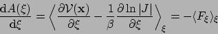
The connection between
the derivative of the free energy with respect to
the reaction coordinate,
![]() ,
and the forces exerted along the latter
may be written as: [24,11]
,
and the forces exerted along the latter
may be written as: [24,11]
where ![]() is the determinant of the Jacobian for the
transformation from generalized to Cartesian coordinates. The
first term of the ensemble average corresponds to the Cartesian
forces exerted on the system, derived from the potential energy
function,
is the determinant of the Jacobian for the
transformation from generalized to Cartesian coordinates. The
first term of the ensemble average corresponds to the Cartesian
forces exerted on the system, derived from the potential energy
function,
![]() . The second contribution is a geometric
correction arising from the change in the metric of the phase
space due to the use of generalized coordinates.
It is worth noting, that, contrary to its instantaneous
component,
. The second contribution is a geometric
correction arising from the change in the metric of the phase
space due to the use of generalized coordinates.
It is worth noting, that, contrary to its instantaneous
component, ![]() , only the average force,
, only the average force,
![]() , is physically meaningful.
, is physically meaningful.
In the framework of the average biasing force (ABF)
approach, [10,20]
![]() is accumulated in small windows
or bins of finite size,
is accumulated in small windows
or bins of finite size, ![]() ,
thereby providing an estimate of the derivative
,
thereby providing an estimate of the derivative
![]() defined in equation (6).
The force applied along the reaction coordinate,
defined in equation (6).
The force applied along the reaction coordinate,
![]() , to overcome free energy barriers is defined
by:
, to overcome free energy barriers is defined
by:
where ![]() denotes the current estimate of the
free energy and
denotes the current estimate of the
free energy and
![]() , the current
average of
, the current
average of ![]() .
.
As sampling of the phase space proceeds, the estimate
![]() is progressively refined. The biasing
force,
is progressively refined. The biasing
force,
![]() , introduced in the equations of
motion guarantees that in the bin centered about
, introduced in the equations of
motion guarantees that in the bin centered about ![]() ,
the force acting along the reaction coordinate averages
to zero over time. Evolution of the system along
,
the force acting along the reaction coordinate averages
to zero over time. Evolution of the system along ![]() is, therefore, governed mainly by its self-diffusion
properties.
is, therefore, governed mainly by its self-diffusion
properties.
A particular feature of the
instantaneous force, ![]() ,
is its tendency to fluctuate
significantly.
As a result, in the beginning of an ABF simulation,
the accumulated average in each bin will generally
take large, inaccurate
values. Under these circumstances,
applying the biasing force along
,
is its tendency to fluctuate
significantly.
As a result, in the beginning of an ABF simulation,
the accumulated average in each bin will generally
take large, inaccurate
values. Under these circumstances,
applying the biasing force along ![]() according
to equation (7) may severely perturb
the dynamics of the system, thereby
biasing artificially the accrued average, and,
thus, impede convergence.
To avoid such undesirable effects,
no biasing force is applied in a bin centered about
according
to equation (7) may severely perturb
the dynamics of the system, thereby
biasing artificially the accrued average, and,
thus, impede convergence.
To avoid such undesirable effects,
no biasing force is applied in a bin centered about ![]() until a reasonable number of force samples
has been collected. When the user-defined minimum number
of samples is reached, the biasing force
is introduced progressively in the form
of a linear ramp.
For optimal efficiency, this minimal number of samples
should be adjusted on a system-dependent basis.
until a reasonable number of force samples
has been collected. When the user-defined minimum number
of samples is reached, the biasing force
is introduced progressively in the form
of a linear ramp.
For optimal efficiency, this minimal number of samples
should be adjusted on a system-dependent basis.
In addition, to alleviate the deleterious
effects caused by abrupt variations of the force,
the corresponding fluctuations are smoothed out,
using a weighted running average over a preset number
of adjacent bins, in lieu of the average of the
current bin itself. It is, however, crucial to ascertain
that the free energy profile varies regularly
in the ![]() -interval, over which the
average is performed.
-interval, over which the
average is performed.
To obtain an adequate sampling in reasonable
simulation times, it is recommended to split long reaction
pathways into consecutive ranges of ![]() . In contrast with
probability-based methods, ABF does
not require that these windows overlap by
virtue of the continuity of the force across the
the reaction pathway.
. In contrast with
probability-based methods, ABF does
not require that these windows overlap by
virtue of the continuity of the force across the
the reaction pathway.
A more comprehensive discussion of the theoretical basis of the method and its implementation in NAMD can be found in [13].
The ABF method has been implemented as a suite of Tcl routines that can be invoked from the main configuration file used to run molecular dynamics simulations with NAMD.
The routines can be invoked by including the following command in the configuration file:
source <path to>/lib/abf/abf.tcl
where <path to>/lib/abf/abf.tcl is the complete path to the main ABF file. The other Tcl files of the ABF package must be located in the same directory.
A second option for loading the ABF module is to source the lib/init.tcl file distributed with NAMD, and then use the Tcl package facility. The file may be sourced in the config file:
source <path to>/lib/init.tcl
package require abf
Or, to make the config file portable, the init file may be the first config file passed to NAMD:
namd2 <path to>/lib/init.tcl myconfig.namd
and then the config file need only contain:
package require abf
Note that the ABF code makes use of the TclForces and TclForcesScript commands. As a result, NAMD configuration files should not call the latter directly when running ABF.
The following parameters have been defined to control ABF calculations. They may be set using the folowing syntax:
where <value> may be a number, a word or a Tcl list. Keywords are not case-sensitive.
|
corresponds to the distance separating two selected
atoms:
abf1: index of the first atom of the reaction coordinate; abf2: index of the second atom of the reaction coordinate. |
|
corresponds to the distance separating the center of
mass of two sets of atoms, e.g.the distance between the
centroid of two benzene molecules:
abf1: list of indices of atoms participating to the first center of mass; abf2: list of indices of atoms participating to the second center of mass. |
|
corresponds to the distance between the centers of mass
of two sets of atoms along a given direction:
direction: a vector (Tcl list of three real numbers) defining the direction of interest abf1: list of indices of atoms participating to the first center of mass; abf2: list of indices of atoms participating to the second center of mass. |
|
corresponds to the distance separating two groups of atoms
along the abf1: list of indices of reference atoms abf2: list of indices of atoms of interest -- e.g.a solute |
|
is similar to zCoord, but using a single
atom of interest
abf1: list of indices of reference atoms abf2: index of an atom of interest |
|
is the distance between the centers of mass of
two atom groups, projected on
the abf1: list of indices of atoms participating to the first center of mass; abf2: list of indices of atoms participating to the second center of mass. |
In close connection with the possibility to run umbrella sampling simulations, the ABF module of NAMD also includes the capability to add sets of restraints to confine the system in selected regions of configurational space. Incorporation of harmonic restraints may be invoked using a syntax similar in spirit to that adopted in the conformational free energy module of NAMD:
abf restraintList {
   angle1  {angle {A 1 CA} {G 1 N3} {G 1 N1}          40.0 30.0}
   dihe1   {dihe  {A 1 O1} {A 1 CA} {A 1 O2} {G 1 N3} 40.0  0.0}
   dihe2   {dihe  {A 1 CA} {A 1 O2} {G 1 N2} {G 1 N3} 40.0  0.0}
}
The general syntax of an item of this list is:
name {type atom1 atom2 [atom3] [atom4] k reference}
where name could be any word used to refer to the restraint in the NAMD output. type is the type of restraint, i.e.a distance, dist, a valence angle, angle, or a dihedral angle, dihe. Definition of the successive atoms follows the syntax of NAMD conformation free energy calculations. k is the force constant of the harmonic restraint, the unit of which depends on type. reference is the reference, target value of the restrained coordinate.
Aside from dist, angle and dihe, which correspond to harmonic restraints, linear ramps have been added for distances, using the specific keyword distLin. In this particular case, generally useful in umbrella sampling free energy calculations, the syntax is:
name {distLin atom1 atom2 F r1 r2}
where F is the force in kcal/mol/Å. The restraint is applied over the interval between r1 and r2.
The harm restraint applies, onto one single atom, a harmonic potential
of the form
This way, atoms may be restrained to the vicinity of a plane, an axis, or a point, depending on the number of nonzero force constants. The syntax is:
name {harm atom {kx ky kz} {x0 y0 z0} }
The formalism implemented in NAMD had been originally devised in the framework of unconstrained MD. Holonomic constraints may, however, be introduced without interfering with the computation of the bias and, hence, the PMF, granted that some precautions are taken.
Either of the following strategies may be adopted:
In some cases, not all atoms used for defining ![]() are involved in
the computation of the force component
are involved in
the computation of the force component ![]() . Specifically, reference
atoms abf1 in the RC types zCoord and zCoord-1atom
are not taken into account in
. Specifically, reference
atoms abf1 in the RC types zCoord and zCoord-1atom
are not taken into account in ![]() . Therefore, constraints involving
those atoms have no effect on the ABF protocol.
. Therefore, constraints involving
those atoms have no effect on the ABF protocol.
For example, if the distance from a methane molecule to the center of mass of a water lamella is studied with the zCoord RC by taking water oxygens as a reference (abf1) and all five atoms of methane as the group of interest (abf2):
In this example,
the system consists of a short,
ten-residue peptide, formed by L-alanine amino acids.
Reversible folding/unfolding of
this peptide is carried out using as a reaction coordinate the carbon
atom of the first and the last carbonyl groups -- ![]() , hence,
corresponds to a a simple interatomic distance, defined by the
keyword distance. The reaction pathway is explored between
12 and 32 Å, i.e., over a distance of 20 Å, in a single window.
The variations of the free energy derivative are soft enough to warrant
the use of bins with a width of 0.2 Å, in which forces are accrued.
, hence,
corresponds to a a simple interatomic distance, defined by the
keyword distance. The reaction pathway is explored between
12 and 32 Å, i.e., over a distance of 20 Å, in a single window.
The variations of the free energy derivative are soft enough to warrant
the use of bins with a width of 0.2 Å, in which forces are accrued.
source                ~/lib/abf/abf.tcl

abf coordinate        distance

abf abf1              4
abf abf2              99

abf dxi               0.2
abf xiMin             12.0
abf xiMax             32.0
abf outFile           deca-alanine.dat
abf fullSamples       500
abf inFiles           {}
abf distFile          deca-alanine.dist
abf dSmooth           0.4
Here, the ABF is applied after 500 samples have been
collected, which, in vacuum, have proven to be sufficient
to get a reasonable estimate of
![]() .
.