


Next: Minimization with new parameters
Up: VMD Tutorial
Previous: Missing Parameter Development
Subsections
Semi-empirical parameter generation: SPARTAN
In this exercise, we'll be using the quantum chemistry software package Spartan to calculate the force field parameters for CYG. To start, type spartan -mesa at the unix command prompt and get ready to build a new molecule by chosing
File: New
You should see the Builder interface. You can build
molecules by selecting atom (and bond) types at the right, and placing
them by clicking on the left portion of the screen. Atoms can be
connected by clicking on the open valences. Start by building CYG,
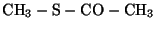 . All the bonds are single except for
the double bond between the carbon and oxygen.
. All the bonds are single except for
the double bond between the carbon and oxygen.
You can turn on atom labels by choosing Model:
Labels. You should have something like this:
Figure 7:
Building CYG in Spartan
![\begin{figure}
\begin{center}
\latex{
\includegraphics[scale=0.5]{FIGS/spart1}
}
\end{center}
\end{figure}](img43.gif) |
Minimize the structure by clicking Minimize at the top. Once it's done, you should see:
Figure 8:
CYG after minimization in Spartan
![\begin{figure}
\begin{center}
\latex{
\includegraphics[scale=0.5]{FIGS/spart2}
}
\end{center}
\end{figure}](img45.gif) |
Return to the main menu by choosing
File: Return to main
Save molecule? Yes
Everything is ready now for a semiempirical quantum mechanics
calculation. You optimize the geometry of the structure, calculate electrostatic
potential (ESP) charges and vibrational frequencies. Finally you perform
a coordinate drive for determining the rotation barrier of one of the
dihedral angles.
From the main menu, choose Setup: Calculations and set the options:
Task: Equilibrium Geometry
Model: Model: Semi-Empirical PM3
Subject to: Symmetry
Compute: Frequencies, Electrostatic Charges
Print: Atomic Charges
Options: check Converge
Figure 9:
Setting up the energy calculation
![\begin{figure}
\begin{center}
\latex{
\includegraphics[scale=0.5]{FIGS/image054}
}
\end{center}
\end{figure}](img46.gif) |
Press Save. You can submit the job and view its output by choosing:
Setup: Submit
Display: Output
The output file lists details about the method used, and lists the Cartesian coordinates of the atoms.
You can measure atomic distances and bond angles by using the
Geometry pulldown.
Next, we are going to display the vibrational modes. The
modes can be viewed through the animation part of the program.
Click: Display: Vibrations; when you check the boxes you
can watch individual vibrational modes. Be sure to increase the
amplitude to see the vibrations clearly.
Figure 10:
Thioester linkage found in 1ODV.pdb, photoactive
yellow protein.
![\begin{figure}
\begin{center}
\latex{
\includegraphics[scale=0.5]{FIGS/thio}
}
\end{center}
\end{figure}](img49.gif) |
A systematic calculation of the force constants for the
bond stretching and angle bending motion can be obtained from the
ab initio calculations [9], but is beyond the scope of
this exercise.
Next, we are going to display a surface around the atoms, on which we will map the ESP charges of the molecule. First check out the numerical values of Mulliken charges and ESP charges and compare the difference between them.
Model: Ball and Wire
Model: Labels
Model: Configure labels
Generally you will see that the partial charge values derived from
an ESP calculation are higher than the Mulliken charges. ESP
charges are calculated to reproduce the electrostatic potential
around an atom, whereas the Mulliken charges are derived from the
electron occupancy of orbitals. ESP charges are usually more
suitable for force field generation.
You can display a potential surface by clicking on Setup: Surfaces.
In the menu, set:
Property: Potential
Add
Figure 11:
Surface set-up
![\begin{figure}
\begin{center}
\latex{
\includegraphics[scale=0.5]{FIGS/image060}
}
\end{center}
\end{figure}](img50.gif) |
Submit the surface calculation with Setup: Submit. When the job completes, you can view the surface with Display: Surfaces.
The next exercise will be to calculate the energy of rotation around the H1-C1-S1-C2 dihedral. In Spartan, this is called a Coordinate Driving calculation (there are other names for the same task, such as conformational sampling, or dihedral search). First we will have to define the dihedral angle of interest:
Build: Define Profile
Figure 12:
Dihedral selection
![\begin{figure}
\begin{center}
\latex{
\includegraphics[scale=0.5]{FIGS/spart4}
}
\end{center}
\end{figure}](img52.gif) |
Select Drive Dihedral. The program expects four continuous atoms to be picked to define the dihedral angle. Click on the same atoms depicted above in the same order.
You will rotate the dihedral angle 360 degrees from its initial value in steps of 15 degrees:
From: initial value
To: initial value + 360
Steps: 24
Return to the File: Main window saving your changes and set up another job with Setup: Calculations, this time choosing
Task: Energy Profile
Figure 13:
Energy profile calculation
![\begin{figure}
\begin{center}
\latex{
\includegraphics[scale=0.5]{FIGS/image068}
}
\end{center}
\end{figure}](img53.gif) |
Submit it with Setup: Submit. It will take several minutes
to run, but you can follow the progress on Display: Output.
After the job is done, you can see the energy for each sampled conformation
by selecting:
Geometry: Measure Dihedral click on same 4 atoms, choose 0 to 360, then click on "ladder-like" button (on right),
then close measure dihedral box
Display: Spreadsheet
Column: Add E_gas: in kcal/mol
Plot these values by selecting Display: Plots: Create, and
choosing Dih360 for the X-axis and E_gas
(kcal/mol) for the Y-axis.
Click anywhere on the function (it will look a bit strange; we will smooth is now)
Display: Plots: Edit Choose Fourier Least Squares
Figure 14:
Dihedral energy profile results after
smoothing, in Spartan
![\begin{figure}
\begin{center}
\latex{
\includegraphics[scale=4.0]{FIGS/spart5new}
}
\end{center}
\end{figure}](img54.gif) |
Next: Minimization with new parameters
Up: VMD Tutorial
Previous: Missing Parameter Development
vmd@ks.uiuc.edu
![\framebox[\textwidth]{
\begin{minipage}{.2\textwidth}
\includegraphics[width...
...he molecule, and shift+right button to scale the molecule.}
\end{minipage}
}](img42.gif)
![\framebox[\textwidth]{
\begin{minipage}{.2\textwidth}
\includegraphics[width...
...e at the right and selecting the atoms or bonds to alter. }
\end{minipage}
}](img44.gif)
![\framebox[\textwidth]{
\begin{minipage}{.2\textwidth}
\includegraphics[width...
... and compare the values with the proposed values from MOE.}
\end{minipage}
}](img47.gif)
![\framebox[\textwidth]{
\begin{minipage}{.2\textwidth}
\includegraphics[width...
...e thioester
linkage for 1ODV.pdb, figure presented below.}
\end{minipage}
}](img48.gif)
![\framebox[\textwidth]{
\begin{minipage}{.2\textwidth}
\includegraphics[width...
...e color scheme on the surface fit the ESP partial charges?}
\end{minipage}
}](img51.gif)
![\framebox[\textwidth]{
\begin{minipage}{.2\textwidth}
\includegraphics[width...
... Where are the minimum and maximum
points of the energy? }
\end{minipage}
}](img55.gif)