


Next: Alchemical Free Energy Methods1
Up: Collective Variable-based Calculations1
Previous: Declaring and using collective
Contents
Index
Subsections
Biasing and analysis methods
All of the biasing and analysis methods implemented (abf,
harmonic, histogram and metadynamics)
recognize the following options:
Adaptive Biasing Force
For a full description of the Adaptive Biasing Force method, see
reference [20]. For details about this implementation,
see references [32] and [33]. When
publishing research that makes use of this functionality, please cite
references [20] and [33].
An alternate usage of this feature is the application of custom
tabulated biasing potentials to one or more colvars. See
inputPrefix and updateBias below.
ABF is based on the thermodynamic integration (TI) scheme for
computing free energy profiles. The free energy as a function
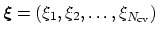
of a set of collective variables
![$ {\mbox{\boldmath {$\xi$}}}=(\xi_{i})_{i\in[1,n]}$](img337.png) is defined from the canonical distribution of
is defined from the canonical distribution of
 ,
,
 :
:
 |
(45) |
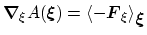
In the TI formalism, the free energy is obtained from its gradient,
which is generally calculated in the form of the average of a force
 exerted on
, taken over an iso-
surface:
exerted on
, taken over an iso-
surface:
 |
(46) |
Several formulae that take the form of (47) have been
proposed. This implementation relies partly on the classic
formulation [14], and partly on a more versatile scheme
originating in a work by Ruiz-Montero et al. [58],
generalized by den Otter [21] and extended to multiple
variables by Ciccotti et al. [17]. Consider a system
subject to constraints of the form
 . Let
(
. Let
(
![$ {\mbox{\boldmath {$v$}}}_{i})_{i\in[1,n]}$](img344.png) be arbitrarily chosen vector fields
(
be arbitrarily chosen vector fields
(
 ) verifying, for all
  ,
,
 , and
, and  :
:
then the following holds [17]:
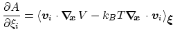 |
(49) |
where  is the potential energy function.
 can be interpreted as the direction along which the force
acting on variable
can be interpreted as the direction along which the force
acting on variable  is measured, whereas the second term in the
average corresponds to the geometric entropy contribution that appears
as a Jacobian correction in the classic formalism [14].
Condition (48) states that the direction along
which the system force on is measured is orthogonal to the
gradient of
is measured, whereas the second term in the
average corresponds to the geometric entropy contribution that appears
as a Jacobian correction in the classic formalism [14].
Condition (48) states that the direction along
which the system force on is measured is orthogonal to the
gradient of  , which means that the force measured on
does not act on .
, which means that the force measured on
does not act on .
Equation (49) implies that constraint forces
are orthogonal to the directions along which the free energy gradient is
measured, so that the measurement is effectively performed on unconstrained
degrees of freedom. In NAMD, constraints are typically applied to the lengths of
bonds involving hydrogen atoms, for example in TIP3P water molecules
(parameter rigidBonds, section 5.6.1).
In the framework of ABF,
 is accumulated in bins of finite size,
 ,
thereby providing an estimate of the free energy gradient
according to equation (47).
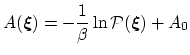
The biasing force applied along the colective variables
to overcome free energy barriers is calculated as:
,
thereby providing an estimate of the free energy gradient
according to equation (47).
The biasing force applied along the colective variables
to overcome free energy barriers is calculated as:
where

 denotes the current estimate of the
free energy gradient at the current point
in the collective
variable subspace.
denotes the current estimate of the
free energy gradient at the current point
in the collective
variable subspace.
As sampling of the phase space proceeds, the estimate
is progressively refined. The biasing
force introduced in the equations of motion guarantees that in
the bin centered around
,
the forces acting along the selected collective variables average
to zero over time. Eventually, as the undelying free energy surface is canceled
by the adaptive bias, evolution of the system along
is governed mainly by diffusion.
Although this implementation of ABF can in principle be used in
arbitrary dimension, a higher-dimension collective variable space is likely
to result in sampling difficulties.
Most commonly, the number of variables is one or two.
ABF requirements on collective variables
- Only linear combinations of colvar components can be used in ABF calculations.
- Availability of system forces is necessary. The following colvar components
can be used in ABF calculations:
distance, distance_xy, distance_z, angle,
dihedral, gyration, rmsd and eigenvector.
Atom groups may not be replaced by dummy atoms, unless they are excluded
from the force measurement by specifying oneSiteSystemForce, if available.
- Mutual orthogonality of colvars. In a multidimensional ABF calculation,
equation (48) must be satisfied for any two colvars and .
Various cases fulfill this orthogonality condition:
- and are based on non-overlapping sets of atoms.
- atoms involved in the force measurement on do not participate in
the definition of . This can be obtained using the option oneSiteSystemForce
of the distance, angle, and dihedral components
(example: Ramachandran angles
 ,
,  ).
).
- and are orthogonal by construction. Useful cases are the sum and
difference of two components, or distance_z and distance_xy using the same axis.
- Mutual orthogonality of components: when several components are combined into a colvar,
it is assumed that their vectors
(equation (50))
are mutually orthogonal. The cases described for colvars in the previous paragraph apply.
- Orthogonality of colvars and constraints: equation 49 can
be satisfied in two simple ways, if either no constrained atoms are involved in the force measurement
(see point 3 above) or pairs of atoms joined by a constraint bond are part of an atom group
which only intervenes through its center (center of mass or geometric center) in the force measurement.
In the latter case, the contributions of the two atoms to the left-hand side of equation 49
cancel out. For example, all atoms of a rigid TIP3P water molecule can safely be included in an atom
group used in a distance component.
The following parameters can be set in the ABF configuration block
(in addition to generic bias parameters such as colvars):
- fullSamples
 (ABF) Number of samples in a bin prior
to application of the ABF
(ABF) Number of samples in a bin prior
to application of the ABF 
Acceptable Values: positive integer
Default Value: 200
Description: To avoid nonequilibrium effects in the dynamics of the system, due to large
fluctuations of the force exerted along the reaction coordinate,  , it
is recommended to apply the biasing force only after a reasonable estimate
of the latter has been obtained.
, it
is recommended to apply the biasing force only after a reasonable estimate
of the latter has been obtained.
- hideJacobian (ABF) Remove geometric entropy term from calculated
free energy gradient?
Acceptable Values: boolean
Default Value: no
Description: In a few special cases, most notably distance-based variables, an alternate definition of
the potential of mean force is traditionally used, which excludes the Jacobian
term describing the effect of geometric entropy on the distribution of the variable.
This results, for example, in particle-particle potentials of mean force being flat
at large separations.
Setting this parameter to yes causes the output data to follow that convention,
by removing this contribution from the output gradients while
applying internally the corresponding correction to ensure uniform sampling.
It is not allowed for colvars with multiple components.
- outputFreq (ABF) Frequency (in timesteps) at which ABF data files are refreshed
Acceptable Values: positive integer
Default Value: Colvar module restart frequency
Description: The files containing the free energy gradient estimate and sampling histogram
(and the PMF in one-dimensional calculations) are written on disk at the given
time interval.
- historyFreq (ABF) Frequency (in timesteps) at which ABF history files are
accumulated
Acceptable Values: positive integer
Default Value: 0
Description: If this number is non-zero, the free energy gradient estimate and sampling histogram
(and the PMF in one-dimensional calculations) are appended to files on disk at
the given time interval. History file names use the same prefix as output files, with
``.hist'' appended.
- inputPrefix (ABF) Filename prefix for reading ABF data
Acceptable Values: list of strings
Description: If this parameter is set, for each item in the list, ABF tries to read
a gradient and a sampling files named inputPrefix.grad
and inputPrefix.count. This is done at
startup and sets the initial state of the ABF algorithm.
The data from all provided files is combined appropriately.
Also, the grid definition (min and max values, width) need not be the same
that for the current run. This command is useful to piece together
data from simulations in different regions of collective variable space,
or change the colvar boundary values and widths. Note that it is not
recommended to use it to switch to a smaller width, as that will leave
some bins empty in the finer data grid.
This option is NOT compatible with reading the data from a restart file
(colvarsInput option of the NAMD config file).
- applyBias (ABF) Apply the ABF bias?
Acceptable Values: boolean
Default Value: yes
Description: If this is set to no, the calculation proceeds normally but the adaptive
biasing force is not applied. Data is still collected to compute
the free energy gradient. This is mostly intended for testing purposes, and should
not be used in routine simulations.
- updateBias (ABF) Update the ABF bias?
Acceptable Values: boolean
Default Value: yes
Description: If this is set to no, the initial biasing force (e.g. read from a restart file or
through inputPrefix) is not updated during the simulation.
As a result, a constant bias is applied. This can be used to apply a custom, tabulated
biasing potential to any combination of colvars. To that effect, one should prepare
a gradient file containing the biasing force to be applied (negative gradient
of the potential), and a count file containing only values greater than
fullSamples. These files must match the grid parameters of the colvars.
ABF also depends on parameters from collective variables to define the grid on which free
energy gradients are computed. In the direction of each colvar, the grid ranges from
lowerBoundary to upperBoundary, and the bin width (grid spacing)
is set by the width parameter.
The ABF bias produces the following files, all in multicolumn ASCII format:
- outputName.grad: current estimate of the free energy gradient (grid),
in multicolumn;
- outputName.count: total number of samples collected, on the same grid;
- outputName.pmf: only for one-dimensional calculations, integrated
free energy profile or PMF.
If several ABF biases are defined concurrently, their name is inserted to produce
unique filenames for output, as in outputName.abf1.grad.
This should not be done routinely and could lead to meaningless results:
only do it if you know what you are doing!
If the colvar space has been partitioned into sections (windows) in which independent
ABF simulations have been run, the resulting data can be merged using the
inputPrefix option described above (a NAMD run of 0 steps is enough).
If a one-dimensional calculation is performed, the estimated free energy
gradient is automatically integrated and a potential of mean force is written
under the file name <outputName>.pmf, in a plain text format that
can be read by most data plotting and analysis programs (e.g. gnuplot).
In dimension 2 or greater, integrating the discretized gradient becomes non-trivial. The
standalone utility abf_integrate is provided to perform that task.
abf_integrate reads the gradient data and uses it to perform a Monte-Carlo (M-C)
simulation in discretized collective variable space (specifically, on the same grid
used by ABF to discretize the free energy gradient).
By default, a history-dependent bias (similar in spirit to metadynamics) is used:
at each M-C step, the bias at the current position is incremented by a preset amount
(the hill height).
Upon convergence, this bias counteracts optimally the underlying gradient;
it is negated to obtain the estimate of the free energy surface.
abf_integrate is invoked using the command-line:
integrate <gradient_file> [-n <nsteps>] [-t <temp>] [-m (0|1)]
                          [-h <hill_height>] [-f <factor>]
The gradient file name is provided first, followed by other parameters in any order.
They are described below, with their default value in square brackets:
- -n: number of M-C steps to be performed; by default, a minimal number of
steps is chosen based on the size of the grid, and the integration runs until a convergence
criterion is satisfied (based on the RMSD between the target gradient and the real PMF gradient)
- -t: temperature for M-C sampling (unrelated to the simulation temperature)
[500 K]
- -m: use metadynamics-like biased sampling? (0 = false) [1]
- -h: increment for the history-dependent bias (``hill height'') [0.01 kcal/mol]
- -f: if non-zero, this factor is used to scale the increment stepwise in the
second half of the M-C sampling to refine the free energy estimate [0.5]
Using the default values of all parameters should give reasonable results in most cases.
abf_integrate produces the following output files:
- <gradient_file>.pmf: computed free energy surface
- <gradient_file>.histo: histogram of M-C sampling (not
usable in a straightforward way if the history-dependent bias has been applied)
- <gradient_file>.est: estimated gradient of the calculated free energy surface
(from finite differences)
- <gradient_file>.dev: deviation between the user-provided numerical gradient
and the actual gradient of the calculated free energy surface. The RMS norm of this vector
field is used as a convergence criteria and displayed periodically during the integration.
Note: Typically, the ``deviation'' vector field does not
vanish as the integration converges. This happens because the
numerical estimate of the gradient does not exactly derive from a
potential, due to numerical approximations used to obtain it (finite
sampling and discretization on a grid).
Metadynamics
Many methods have been introduced in the past that make use of an
artificial energy term, that changes and adapts over time, to
reconstruct a potential of mean force from a conventional molecular
dynamics simulation [34,27,71,19,42,35]. One of the most recent,
metadynamics, was first designed as a stepwise algorithm, which may
be roughly described as an ``adaptive umbrella sampling''
[42], and was later made continuous over time
[36]. This implementation provides only he latter
version, which is the most commonly used.
In metadynamics, the external potential on the colvars
 is:
is:
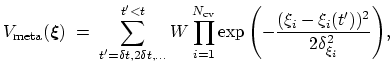 |
(51) |
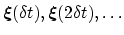
that is,
 is a history-dependent potential,
which acts on the current values of the colvars
and
depends parametrically on the previous values of the colvars. It is
constructed as a sum of
is a history-dependent potential,
which acts on the current values of the colvars
and
depends parametrically on the previous values of the colvars. It is
constructed as a sum of
 -dimensional repulsive
Gaussian ``hills'' with a height
-dimensional repulsive
Gaussian ``hills'' with a height  : their centers are located at the
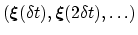
previously explored configurations
: their centers are located at the
previously explored configurations
 , and they extend by
approximately
, and they extend by
approximately
 in the direction of the -th
colvar.
in the direction of the -th
colvar.
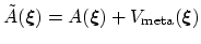
As the system evolves according to the underlying potential of mean
force
 incremented by the metadynamics potential
 , new hills will tend to accumulate in
the regions with a lower effective free energy
, new hills will tend to accumulate in
the regions with a lower effective free energy
 . That is, the probability of
having a given system configuration
. That is, the probability of
having a given system configuration
 being explored (and
thus, a hill being added there) is proportional to
being explored (and
thus, a hill being added there) is proportional to
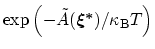 ,
which tends to a nearly flat histogram when the simulation is
continued until the system has deposited hills across the whole free
energy landscape. In this situation,
,
which tends to a nearly flat histogram when the simulation is
continued until the system has deposited hills across the whole free
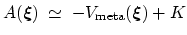
energy landscape. In this situation,
 is a good approximant of the free energy
, and the only
dependence on the specific conformational history
is a good approximant of the free energy
, and the only
dependence on the specific conformational history
 is by an
irrelevant additive constant:
is by an
irrelevant additive constant:
 |
(52) |
Provided that the set of collective variables fully describes the
relevant degrees of freedom, the accuracy of the reconstructed profile
is a function of the ratio between and  [13]. For the optimal choice of
 and
and
 , the diffusion constant of the variable , see
reference [13]. As a rule of thumb, the very upper limit
for the ratio
, the diffusion constant of the variable , see
reference [13]. As a rule of thumb, the very upper limit
for the ratio
 is given by
 , where
 is the
longest among
's correlation times. In the most typical
conditions, to achieve a good statistical convergence the user would
prefer to keep
much smaller than
.
is the
longest among
's correlation times. In the most typical
conditions, to achieve a good statistical convergence the user would
prefer to keep
much smaller than
.
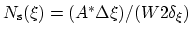
Given  the extension of the free energy profile along the
colvar , and
the extension of the free energy profile along the
colvar , and
 the highest free energy that
needs to be sampled (e.g. that of a transition state), the upper bound
for the required simulation time is of the order of
the highest free energy that
needs to be sampled (e.g. that of a transition state), the upper bound
for the required simulation time is of the order of
 multiples of
. When several colvars
are used, the upper
bound amounts to
multiples of
. When several colvars
are used, the upper
bound amounts to
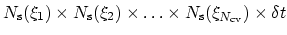 .
.
In metadynamics runs performed with this module, the parameter
for each hill (eq. 52) is
chosen as approximately half the width of the corresponding
colvar , while all the other parameters must be provided within
the metadynamics {...} block.
The only mandatory parameter is the colvars option, listing all
the variables to which this bias is applied. Note:
multidimensional PMFs are obtained with one metadynamics
instance applied to all the colvars, and not with multiple instances
applied to individual colvars.
The following two options have default values that are reasonable in
typical situations, but it is strongly recommended that the user chooses
them according to the above discussion on the diffusion times of the
variables,
:
The following options define the configuration for the ``well-tempered'' metadynamics approach [4]:
The following options control the performance of metadynamics
calculations, but do not affect the results:
The following options define metadynamics calculations with more than
one replica:
- multipleReplicas (metadynamics) Multiple replicas metadynamics
Acceptable Values: boolean
Default Value: off
Description: If this option is on, multiple (independent) replica of the
same system can be run at the same time, and their hills will be
combined to obtain a single PMF [56]. Replicas are
identified by the value of replicaID. Communication is
done by files: each replica of NAMD must be able to read the files
created by the others, whose paths are communicated through the file
replicasRegistry. This file, and the files listed in it,
are read every replicaUpdateFrequency steps. Every time
the colvars state file is written
(colvarsRestartFrequency), the file
``outputName.colvars.name.replicaID.state'' is also written, containing
the state of the metadynamics bias for replicaID. In the
time steps between colvarsRestartFrequency, new hills are
temporarily written to the file ``outputName.colvars.name.replicaID.hills'', which serves as communication
buffer. These files are only required for communication, and may be
deleted after a new NAMD run is started with a different
outputName.
- replicaID (metadynamics) Set the identifier for this replica
Acceptable Values: string
Description: If multipleReplicas is on, this option sets a
unique identifier for this replica. All replicas should use
identical collective variable configurations, except for the value
of this option.
- replicasRegistry (metadynamics) Multiple replicas database file
Acceptable Values: UNIX filename
Default Value: ``name.replica_files.txt''
Description: If multipleReplicas is on, this option sets the
path to the replicas' database file.
- replicaUpdateFrequency (metadynamics) How often hills are communicated between
replicas
Acceptable Values: positive integer
Default Value: newHillFrequency
Description: If multipleReplicas is on, this option sets the
number of steps after which each replica (re)reads the other
replicas' files. The lowest meaningful value of this number is
newHillFrequency. If access to the file system is
significantly affecting the simulation performance, this number can
be increased, at the price of reduced synchronization between
replicas. Values higher than colvarsRestartFrequency may
not improve performance significantly.
- dumpPartialFreeEnergyFile (metadynamics) Periodically write the contribution to the
PMF from this replica
Acceptable Values: boolean
Default Value: on
Description: When multipleReplicas is on, tje file
outputName.pmf contains the combined PMF from all
replicas. Enabling this option will produce an additional file
outputName.partial.pmf, which can be useful to
quickly monitor the contribution of each replica to the PMF. The
requirements for this option are the same as
dumpFreeEnergyFile.
The following options may be useful for applications that go beyond the
direct application of metadynamics for a calculation of a PMF.
- name (metadynamics) Name of this metadynamics instance
Acceptable Values: string
Default Value: ``meta'' + rank number
Description: This option sets the name for this metadynamics instance. While it
is not advisable to use more than one metadynamics instance within
the same simulation, this allows to distinguish each instance from
the others. If there is more than one metadynamics instance, the
name of this bias is included in the metadynamics output file names
such as dumpFreeEnergyFile.
- saveFreeEnergyFile (metadynamics) Keep all the PMF files
Acceptable Values: boolean
Default Value: off
Description: When dumpFreeEnergyFile and this option are on,
the step number is included in the file name. Activating this
option can be useful to follow more closely the convergence of the
simulation, by comparing PMFs separated by short times.
- keepHills (metadynamics) Write each individual hill to the state
file
Acceptable Values: boolean
Default Value: off
Description: When useGrids and this option are on, all hills
are saved to the state file in their analytic form, alongside their
grids. This makes it possible to later use exact analytic Gaussians
for rebinGrids. To only keep track of the history of the
added hills, writeHillsTrajectory is preferable.
- writeHillsTrajectory (metadynamics) Write a log of new hills
Acceptable Values: boolean
Default Value: on
Description: If this option is on, a logfile is written by the
metadynamics bias, with the name
``outputName.colvars.name.hills.traj'', which
can be useful to follow the time series of the hills. When
multipleReplicas is on, its name changes to
``outputName.colvars.name.replicaID.hills.traj''.
This file can be used to quickly visualize the positions of all
added hills, in case newHillFrequency does not coincide
with colvarsRestartFrequency.
Harmonic restraints and Steered Molecular Dynamics
The harmonic biasing method may be used to enforce fixed or moving restraints,
including variants of Steered and Targeted MD. Within energy minimization
runs, it allows for restrained minimization, e.g. to calculate relaxed potential
energy surfaces. In the context of the colvars module,
harmonic potentials are meant according to their textbook definition:
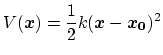 .
Note that this differs from harmonic bond and angle potentials in common
force fields, where the factor of one half is typically omitted,
resulting in a non-standard definition of the force constant.
The restraint energy is reported by NAMD under the MISC title.
A harmonic restraint is set up by a harmonic {...}
block, which may contain (in addition to the standard option
colvars) the following keywords:
.
Note that this differs from harmonic bond and angle potentials in common
force fields, where the factor of one half is typically omitted,
resulting in a non-standard definition of the force constant.
The restraint energy is reported by NAMD under the MISC title.
A harmonic restraint is set up by a harmonic {...}
block, which may contain (in addition to the standard option
colvars) the following keywords:
- forceConstant (harmonic) Scaled force constant (kcal/mol)
Acceptable Values: positive decimal
Default Value: 1.0
Description: This defines a scaled force constant for the harmonic potential.
To ensure consistency for multidimensional restraints, it is
divided internally by the square of the specific width
for each colvar involved (which is 1 by default), so that all colvars
are effectively dimensionless and of commensurate size.
For instance, setting a scaled force constant of 10 kcal/mol acting
on two colvars, an angle with a width of 5 degrees and a distance
with a width of 0.5 Å, will apply actual force constants of
0.4 kcal/mol degree
 for the angle and
40 kcal/mol/Å
for the angle and
40 kcal/mol/Å for the distance.
- centers (harmonic) Initial harmonic restraint centers
Acceptable Values: space-separated list of colvar values
Description: The centers (equilibrium values) of the restraint are entered here.
The number of values must be the number of requested colvars.
Each value is a decimal number if the corresponding colvar returns
a scalar, a ``(x, y, z)'' triplet if it returns a unit
vector or a vector, and a ``(q0, q1, q2, q3)'' quadruplet
if it returns a rotational quaternion. If a colvar has
periodicities or symmetries, its closest image to the restraint
center is considered when calculating the harmonic potential.
- targetCenters (harmonic) Steer the restraint centers towards these
targets
Acceptable Values: space-separated list of colvar values
Description: When defined, the current centers will be moved towards
these values during the simulation.
By default, the centers are moved over a total of
targetNumSteps steps by a linear interpolation, in the
spirit of Steered MD.
If targetNumStages is set to a nonzero value, the
change is performed in discrete stages, lasting targetNumSteps
steps each. This second mode may be used to sample successive
windows in the context of an Umbrella Sampling simulation.
When continuing a simulation
run, the centers specified in the configuration file
colvarsConfig will be overridden by those saved in
the restart file colvarsInput. To perform Steered
MD in an arbitrary space of colvars, it is
sufficient to use this option and enable
outputAppliedForce within each of the colvars involved.
- targetForceConstant (harmonic) Change the force constant towards this value
Acceptable Values: positive decimal
Description: When defined, the current forceConstant will be moved towards
this value during the simulation. Time evolution of the force constant
is dictated by the targetForceExponent parameter (see below).
By default, the force constant is changed smoothly over a total of
targetNumSteps steps. This is useful to introduce or
remove restraints in a progressive manner.
If targetNumStages is set to a nonzero value, the
change is performed in discrete stages, lasting targetNumSteps
steps each. This second mode may be used to compute the
conformational free energy change associated with the restraint, within
the FEP or TI formalisms. For convenience, the code provides an estimate
of the free energy derivative for use in TI. A more complete free energy
calculation (particularly with regard to convergence analysis),
while not handled by the colvars module, can be performed by post-processing
the colvars trajectory, if colvarsTrajFrequency is set to a
suitably small value. It should be noted, however, that restraint
free energy calculations may be handled more efficiently by an
indirectly route, through the
determination of a PMF for the restrained coordinate.[22]
- targetForceExponent Exponent in the time-dependence of the force constant
Acceptable Values: decimal equal to or greater than 1.0
Default Value: 1.0
Description: Sets the exponent,  , in the function used to vary the force
constant as a function of time. The force is varied according to a
coupling parameter
, in the function used to vary the force
constant as a function of time. The force is varied according to a
coupling parameter  , raised to the power :
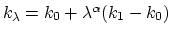 , where
  ,
,
 , and
, and  are the initial, current, and final values
of the force constant. The parameter evolves linearly from
0 to 1, either smoothly, or in targetNumStages equally spaced
discrete stages, or according to an arbitrary schedule set with
lambdaSchedule.
When the initial value of the force constant is zero,
an exponent greater than 1.0 distributes the effects of introducing the
restraint more smoothly over time than a linear dependence, and
ensures that there is no singularity in the derivative of the
restraint free energy with respect to lambda. A value of 4 has
been found to give good results in some tests.
are the initial, current, and final values
of the force constant. The parameter evolves linearly from
0 to 1, either smoothly, or in targetNumStages equally spaced
discrete stages, or according to an arbitrary schedule set with
lambdaSchedule.
When the initial value of the force constant is zero,
an exponent greater than 1.0 distributes the effects of introducing the
restraint more smoothly over time than a linear dependence, and
ensures that there is no singularity in the derivative of the
restraint free energy with respect to lambda. A value of 4 has
been found to give good results in some tests.
- targetNumSteps (harmonic) Number of steps for steering
Acceptable Values: positive integer
Description: Defines the number of steps required to
move the restraint centers (or force constant) towards the values
specified with targetCenters or targetForceConstant.
After the target values have been reached, the centers (resp. force
constant) are kept fixed.
- targetEquilSteps (harmonic) Number of steps discarded from TI estimate
Acceptable Values: positive integer
Description: Defines the number of steps within each stage that are considered
equilibration and discarded from the restraint free energy derivative
estimate reported reported in the output.
- targetNumStages (harmonic) Number of stages for steering
Acceptable Values: non-negative integer
Default Value: 0
Description: If non-zero, sets the number of stages in which the restraint centers
or force constant are changed to their target values. If zero, the change
is continuous.
- lambdaSchedule (harmonic) Schedule of lambda-points for changing force constant
Acceptable Values: list of real numbers between 0 and 1
Description: If specified together with targetForceConstant, sets the sequence of
discrete values that will be used for different stages.
Tip: A complex set of restraints can be applied to a system,
by defining several colvars, and applying one or more harmonic
restraints to different groups of colvars. In some cases, dozens of
colvars can be defined, but their value may not be relevant: to
limit the size of the colvars trajectory file, it
may be wise to disable outputValue for such ``ancillary''
variables, and leave it enabled only for ``relevant'' ones.
Multidimensional histograms
The histogram feature is used to record the distribution of a set of collective
variables in the form of a N-dimensional histogram.
It functions as a ``collective variable bias'', and is invoked by adding a
histogram block to the colvars configuration file.
In addition to the common parameters name and colvars
described above, a histogram block may define the following parameter:
- outputFreq (histogram) Frequency (in timesteps) at which the histogram file is refreshed
Acceptable Values: positive integer
Default Value: Colvar module restart frequency
Description: The file containing histogram data is written on disk at the given time interval.
Like the ABF and metadynamics biases, histogram uses
parameters from the colvars to define its grid. The grid ranges from
lowerBoundary to upperBoundary, and the bin width is
set by the width parameter.
Next: Alchemical Free Energy Methods1
Up: Collective Variable-based Calculations1
Previous: Declaring and using collective
Contents
Index
http://www.ks.uiuc.edu/Research/namd/