


Next: Biasing and analysis methods
Up: Collective Variable-based Calculations1
Previous: General parameters and input/output
Contents
Index
Subsections
Declaring and using collective variables
Each collective variable (colvar) is defined as a combination of one
or more individual quantities, called components (see
Figure 6). In most applications, only one is
needed: in this case, the colvar and its component may be identified.
In the configuration file, each colvar is created by the keyword
colvar, followed by its configuration options, usually
between curly braces, colvar {...}. Each component is
defined within the the colvar {...} block, with a specific
keyword that identifies the functional form: for example,
distance {...} defines a component of the type ``distance
between two atom groups''.
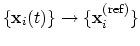
To obtain the value of the colvar,
 , its components
 are summed with the formula:
![$\displaystyle \xi(\mathbf{r}) = \sum_i c_i [q_i(\mathbf{r})]^{n_i}$](img244.png) |
(36) |
where each component appears with a unique coefficient  (1.0 by
default) the positive integer exponent
(1.0 by
default) the positive integer exponent  (1 by default).
For information on setting these parameters, see 10.2.3.
(1 by default).
For information on setting these parameters, see 10.2.3.
- name
 (colvar) Name of this colvar
Acceptable Values: string
Default Value: ``colvar'' + numeric id
Description: The name is an unique case-sensitive string which allows the
colvar module to identify this colvar unambiguously; it is also
used in the trajectory file to label to the columns corresponding
to this colvar.
- width (colvar) Typical fluctuation amplitude (or grid
spacing)
Acceptable Values: positive decimal
Default Value: 1.0
Description: This number is a user-provided estimate of the typical
fluctuation amplitude for this collective variable, or conversely,
the typical width of a local free energy basin. Typically, twice
the standard deviation during a very short simulation run can be
used. Biasing methods use this parameter for different purposes:
harmonic restraints (10.3.3) use it to
rescale the value of this colvar, the histogram
(10.3.4) and ABF biases
(10.3.1) interpret it as the grid spacing in the
direction of this variable, and metadynamics
(10.3.2) uses it to set the width of newly
added hills. This number is expressed in the same physical unit
as the colvar value.
- lowerBoundary (colvar) Lower boundary of the colvar
Acceptable Values: decimal
Description: Defines the lowest possible value in the domain of values that
this colvar can access. It can either be the true lower physical
boundary (under which the variable is not defined by
construction), or an arbitrary value set by the user. Together
with upperBoundary and width, it provides
initial parameters to define grids of values for the colvar. This
option is not available for those colvars that return non-scalar
values (i.e. those based on the components distanceDir
or orientation).
- upperBoundary (colvar) Upper boundary of the colvar
Acceptable Values: decimal
Description: Similarly to lowerBoundary, defines the highest possible
or allowed value.
- expandBoundaries (colvar) Allow biases to expand the two boundaries
Acceptable Values: boolean
Default Value: off
Description: If defined, biasing and analysis methods may keep their own copies
of lowerBoundary and upperBoundary, and expand
them to accommodate values that do not fit in the initial range.
Currently, this option is used by the metadynamics bias
(10.3.2) to keep all of its hills fully within
the grid. Note: this option cannot be used when
the initial boundaries already span the full period of a periodic
colvar.
- extendedLagrangian (colvar) Add extended degree of freedom
Acceptable Values: boolean
Default Value: off
Description: Adds a fictitious particle to be coupled to the colvar by a harmonic
spring. The fictitious mass and the force constant of the coupling
potential are derived from the parameters extendedTimeConstant
and extendedFluctuation, described below. Biasing forces on the
colvar are applied to this fictitious particle, rather than to the
atoms directly. This implements the extended Lagrangian formalism
used in some metadynamics simulations [36].
The energy associated with the extended degree of freedom is reported
under the MISC title in NAMD's energy output.
- extendedFluctuation (colvar) Standard deviation between the colvar and the fictitious
particle (colvar unit)
Acceptable Values: positive decimal
Default Value: 0.2  width
width
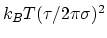
Description: Defines the spring stiffness for the extendedLagrangian
mode, by setting the typical deviation between the colvar and the extended
degree of freedom due to thermal fluctuation.
The spring force constant is calculated internally as
 ,
where
,
where  is the value of extendedFluctuation.
- extendedTimeConstant (colvar) Oscillation period of the fictitious particle (fs)
Acceptable Values: positive decimal
Default Value: 40.0 timestep
Description: Defines the inertial mass of the fictitious particle, by setting the
oscillation period of the harmonic oscillator formed by the fictitious
particle and the spring. The period
should be much larger than the MD time step to ensure accurate integration
of the extended particle's equation of motion.
The fictitious mass is calculated internally as
 ,
where
,
where  is the period and is the typical fluctuation (see above).
- extendedTemp (colvar) Temperature for the extended degree of freedom (K)
Acceptable Values: positive decimal
Default Value: NAMD thermostat temperature
Description: Temperature used for calculating the coupling force constant of the
extended coordinate (see extendedFluctuation) and, if needed, as a
target temperature for extended Langevin dynamics (see
extendedLangevinDamping). This should normally be left at its
default value.
- extendedLangevinDamping (colvar) Damping factor for extended Langevin dynamics
(ps
 )
)
Acceptable Values: positive decimal
Default Value: 0.0
Description: If this is non-zero, the extended degree of freedom undergoes Langevin dynamics
at temperature extendedTemp. The friction force is minus
extendedLangevinDamping times the velocity. This might be useful in
cases where the extended dynamics tends to become unstable because of resonances
with other degrees of freedom. Only use when strictly necessary, as it adds
viscous friction (potentially slowing down diffusive sampling) and stochastic
noise (increasing the variance of statistical measurements).
Collective variable components
Each colvar is defined by one or more components (typically
only one). Each component consists of a keyword identifying a
functional form, and a definition block following that keyword,
specifying the atoms involved and any additional parameters (cutoffs,
``reference'' values, ...).
The types of the components used in a colvar determine the properties
of that colvar, and which biasing or analysis methods can be applied.
In most cases, the colvar returns a real number, which is computed by
one or more instances of the following components:
- distance: distance between two groups;
- distanceZ: projection of a distance vector on an axis;
- distanceXY: projection of a distance vector on a plane;
- distanceVec: distance vector between two groups;
- distanceDir: unit vector parallel to distanceVec;
- angle: angle between three groups;
- coordNum: coordination number between two groups;
- selfCoordNum: coordination number of atoms within a
group;
- hBond: hydrogen bond between two atoms;
- rmsd: root mean square deviation (RMSD) from a set of
reference coordinates;
- eigenvector: projection of the atomic coordinates on a
vector;
- orientationAngle: angle of the best-fit rotation from
a set of reference coordinates;
- tilt: projection on an axis of the best-fit rotation
from a set of reference coordinates;
- gyration: radius of gyration of a group of atoms;
- alpha:
 -helix content of a protein segment.
- dihedralPC: projection of protein backbone dihedrals onto a dihedral principal component.
The following components returns
real numbers that lie in a periodic interval:
- dihedral: torsional angle between four groups;
- spinAngle: angle of rotation around a predefined axis
in the best-fit from a set of reference coordinates.
In certain conditions, distanceZ can also be periodic, namely
when periodic boundary conditions (PBCs) are defined in the simulation
and distanceZ's axis is parallel to a unit cell vector.
The following keywords can be used within periodic components (and are
illegal elsewhere):
Internally, all differences between two values of a periodic colvar
follow the minimum image convention: they are calculated based on
the two periodic images that are closest to each other.
Note: linear or polynomial combinations of periodic components
may become meaningless when components cross the periodic boundary.
Use such combinations carefully: estimate the range of possible values
of each component in a given simulation, and make use of
wrapAround to limit this problem whenever possible.
When one of the following are
used, the colvar returns a value that is not a scalar number:
- distanceVec: 3-dimensional vector of the distance
between two groups;
- distanceDir: 3-dimensional unit vector of the distance
between two groups;
- orientation: 4-dimensional unit quaternion representing
the best-fit rotation from a set of reference coordinates.
The distance between two 3-dimensional unit vectors is computed as the
angle between them. The distance between two quaternions is computed
as the angle between the two 4-dimensional unit vectors: because the
orientation represented by
 is the same as the one
represented by
is the same as the one
represented by
 , distances between two quaternions are
computed considering the closest of the two symmetric images.
, distances between two quaternions are
computed considering the closest of the two symmetric images.
Non-scalar components carry the following restrictions:
- Calculation of system forces (outputSystemForce option)
is currently not implemented.
- Each colvar can only contain one non-scalar component.
- Binning on a grid (abf, histogram and
metadynamics with useGrids enabled) is currently
not implemented for colvars based on such components.
Note: while these restrictions apply to individual colvars based
on non-scalar components, no limit is set to the number of scalar
colvars. To compute multi-dimensional histograms and PMFs, use sets
of scalar colvars of arbitrary size.
In addition to the
restrictions due to the type of value computed (scalar or non-scalar),
a final restriction can arise when calculating system force
(outputSystemForce option or application of a abf
bias). System forces are available currently only for the following
components: distance, distanceZ,
distanceXY, angle, dihedral, rmsd,
eigenvector and gyration.
Most components make
use of one or more atom groups, whose syntax of definition is
by their name followed by a definition block like
atoms {...}, or group1 {...} and
group2 {...}. The contents of an atom group block are
described in 10.2.4.
In the following, all the available component types are listed, along
with their physical units and the limiting values, if any. Such
limiting values can be used to define lowerBoundary and
upperBoundary in the parent colvar.
The distance {...} block defines a distance component,
between two atom groups, group1 and group2.
- group1 (distance) First group of atoms
Acceptable Values: Block group1 {...}
Description: First group of atoms.
- group2 (distance) Second group of atoms
Acceptable Values: Block group2 {...}
Description: Second group of atoms.
- forceNoPBC (distance) Calculate absolute rather than minimum-image distance?
Acceptable Values: boolean
Default Value: no
Description: By default, in calculations with periodic boundary conditions, the
distance component returns the distance according to the
minimum-image convention. If this parameter is set to yes,
PBC will be ignored and the distance between the coordinates as maintained
internally will be used. This is only useful in a limited number of
special cases, e.g. to describe the distance between remote points
of a single macromolecule, which cannot be split across periodic cell
boundaries, and for which the minimum-image distance might give the
wrong result because of a relatively small periodic cell.
- oneSiteSystemForce (distance) Measure system force on group 1 only?
Acceptable Values: boolean
Default Value: no
Description: If this is set to yes, the system force is measured along
a vector field (see equation (50) in
section 10.3.1) that only involves atoms of
group1. This option is only useful for ABF, or custom
biases that compute system forces. See
section 10.3.1 for details.
The value returned is a positive number (in Å), ranging from 0
to the largest possible interatomic distance within the chosen
boundary conditions (with PBCs, the minimum image convention is used
unless the forceNoPBC option is set).
The distanceZ {...} block defines a distance projection
component, which can be seen as measuring the distance between two
groups projected onto an axis, or the position of a group along such
an axis. The axis can be defined using either one reference group and
a constant vector, or dynamically based on two reference groups.
- main (distanceZ, distanceXY) Main group of atoms
Acceptable Values: Block main {...}
Description: Group of atoms whose position
 is measured.
- ref (distanceZ, distanceXY) Reference group of
atoms
Acceptable Values: Block ref {...}
Description: Reference group of atoms. The position of its center of mass is
noted
 below.
- ref2 (distanceZ, distanceXY) Secondary reference
group
Acceptable Values: Block ref2 {...}
Default Value: none
Description: Optional group of reference atoms, whose position
 can
be used to define a dynamic projection axis:
can
be used to define a dynamic projection axis:
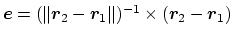 . In this case,
the origin is
. In this case,
the origin is
 , and the value
of the component is
, and the value
of the component is
 .
.
- axis (distanceZ, distanceXY) Projection axis (Å)
Acceptable Values: (x, y, z) triplet
Default Value: (0.0, 0.0, 1.0)
Description: The three components of this vector define (when normalized) a
projection axis
 for the distance vector
 joining the centers of groups ref and
main. The value of the component is then
joining the centers of groups ref and
main. The value of the component is then
 . The vector should be written as three
components separated by commas and enclosed in parentheses.
. The vector should be written as three
components separated by commas and enclosed in parentheses.
- forceNoPBC (distanceZ, distanceXY) Calculate absolute rather than minimum-image distance?
Acceptable Values: boolean
Default Value: no
Description: This parameter has the same meaning as that described above for the distance
component.
- oneSiteSystemForce (distanceZ, distanceXY) Measure system force on group main only?
Acceptable Values: boolean
Default Value: no
Description: If this is set to yes, the system force is measured along a
vector field (see equation (50) in
section 10.3.1) that only involves atoms of main.
This option is only useful for ABF, or custom biases that compute
system forces. See section 10.3.1 for details.
This component returns a number (in Å) whose range is determined
by the chosen boundary conditions. For instance, if the  axis is
used in a simulation with periodic boundaries, the returned value ranges
between
axis is
used in a simulation with periodic boundaries, the returned value ranges
between  and
and  , where
  is the box length
along (this behavior is disabled if forceNoPBC is set).
is the box length
along (this behavior is disabled if forceNoPBC is set).
The distanceXY {...} block defines a distance projected on
a plane, and accepts the same keywords as distanceZ, i.e.
main, ref, either ref2 or axis,
and oneSiteSystemForce. It returns the norm of the
projection of the distance vector between main and
ref onto the plane orthogonal to the axis. The axis is
defined using the axis parameter or as the vector joining
ref and ref2 (see distanceZ above).
The distanceVec {...} block defines
a distance vector component, which accepts the same keywords as
distance: group1, group2, and
forceNoPBC. Its value is the 3-vector joining the centers
of mass of group1 and group2.
The distanceDir {...} block defines
a distance unit vector component, which accepts the same keywords as
distance: group1, group2, and
forceNoPBC. It returns a
3-dimensional unit vector
 , with
 .
.
The angle {...} block defines an angle, and contains the
three blocks group1, group2 and group3, defining
the three groups. It returns an angle (in degrees) within the
interval ![$ [0:180]$](img270.png) .
.
The dihedral {...} block defines a torsional angle, and
contains the blocks group1, group2, group3
and group4, defining the four groups. It returns an angle
(in degrees) within the interval
![$ [-180:180]$](img271.png) . The colvar module
calculates all the distances between two angles taking into account
periodicity. For instance, reference values for restraints or range
boundaries can be defined by using any real number of choice.
. The colvar module
calculates all the distances between two angles taking into account
periodicity. For instance, reference values for restraints or range
boundaries can be defined by using any real number of choice.
- oneSiteSystemForce (angle, dihedral) Measure system force on group 1 only?
Acceptable Values: boolean
Default Value: no
Description: If this is set to yes, the system force is measured along
a vector field (see equation (50) in
section 10.3.1) that only involves atoms of
group1. See section 10.3.1 for an
example.
The coordNum {...} block defines
a coordination number (or number of contacts), which calculates the
function
 , where
  is the
``cutoff'' distance, and
is the
``cutoff'' distance, and  and
and  are exponents that can control
its long range behavior and stiffness [36]. This
function is summed over all pairs of atoms in group1 and
group2:
are exponents that can control
its long range behavior and stiffness [36]. This
function is summed over all pairs of atoms in group1 and
group2:
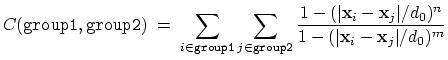 |
(37) |
This colvar component accepts the same keywords as distance,
group1 and group2. In addition to them, it
recognizes the following keywords:
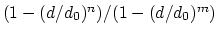
- cutoff (coordNum) ``Interaction'' distance (Å)
Acceptable Values: positive decimal
Default Value: 4.0
Description: This number defines the switching distance to define an
interatomic contact: for  , the switching function
is close to 1, at
, the switching function
is close to 1, at  it
has a value of
it
has a value of  (
( with the default and ), and at
 it goes to zero approximately like
  . Hence,
for a proper behavior, must be larger than .
. Hence,
for a proper behavior, must be larger than .
- expNumer (coordNum) Numerator exponent
Acceptable Values: positive even integer
Default Value: 6
Description: This number defines the exponent for the switching function.
- expDenom (coordNum) Denominator exponent
Acceptable Values: positive even integer
Default Value: 12
Description: This number defines the exponent for the switching function.
- cutoff3 (coordNum) Reference distance vector (Å)
Acceptable Values: ``(x, y, z)'' triplet of positive decimals
Default Value: (4.0, 4.0, 4.0)
Description: The three components of this vector define three different cutoffs
 for each direction. This option is mutually exclusive with
cutoff.
for each direction. This option is mutually exclusive with
cutoff.
- group2CenterOnly (coordNum) Use only group2's center of
mass
Acceptable Values: boolean
Default Value: off
Description: If this option is on, only contacts between the atoms in
group1 and the center of mass of group2 are
calculated. By default, the sum extends over all pairs of
atoms in group1 and group2.
This component returns a dimensionless number, which ranges from
approximately 0 (all interatomic distances much larger than the
cutoff) to
 (all distances
within the cutoff), or
(all distances
within the cutoff), or
 if
group2CenterOnly is used. For performance reasons, at least
one of group1 and group2 should be of limited size
(unless group2CenterOnly is used), because the cost of the
loop over all pairs grows as
.
if
group2CenterOnly is used. For performance reasons, at least
one of group1 and group2 should be of limited size
(unless group2CenterOnly is used), because the cost of the
loop over all pairs grows as
.
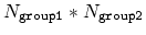
The selfCoordNum {...} block defines
a coordination number in much the same way as coordNum,
but the function is summed over atom pairs within group1:
 |
(38) |
The keywords accepted by selfCoordNum are a subset of
those accepted by coordNum, namely group1
(here defining all of the atoms to be considered),
cutoff, expNumer, and expDenom.
This component returns a dimensionless number, which ranges from
approximately 0 (all interatomic distances much larger than the
cutoff) to
 (all
distances within the cutoff). For performance reasons,
group1 should be of limited size, because the cost of the
loop over all pairs grows as
(all
distances within the cutoff). For performance reasons,
group1 should be of limited size, because the cost of the
loop over all pairs grows as
 .
.
The hBond {...} block defines a hydrogen
bond, implemented as a coordination number (eq. 37)
between the donor and the acceptor atoms. Therefore, it accepts the
same options cutoff (with a different default value of
3.3 Å), expNumer (with a default value of 6) and
expDenom (with a default value of 8). Unlike
coordNum, it requires two atom numbers, acceptor and
donor, to be defined. It returns an adimensional number,
with values between 0 (acceptor and donor far outside the cutoff
distance) and 1 (acceptor and donor much closer than the cutoff).
The block
rmsd {...} defines the root mean square replacement
(RMSD) of a group of atoms with respect to a reference structure. For
each set of coordinates
 , the colvar component rmsd calculates the
optimal rotation
, the colvar component rmsd calculates the
optimal rotation
 that best superimposes the coordinates
 onto a
set of reference coordinates
onto a
set of reference coordinates
 .
Both the current and the reference coordinates are centered on their
centers of geometry,
.
Both the current and the reference coordinates are centered on their
centers of geometry,
 and
and
 . The root mean square
displacement is then defined as:
. The root mean square
displacement is then defined as:
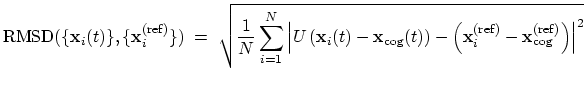 |
(39) |
The optimal rotation
is calculated within the formalism developed in
reference [18], which guarantees a continuous
dependence of
with respect to
. The options for rmsd
are:
- atoms (rmsd) Atom group
Acceptable Values: atoms {...} block
Description: Defines the group of atoms of which the RMSD should be calculated.
- refPositions (rmsd) Reference coordinates
Acceptable Values: space-separated list of (x, y, z) triplets
Description: This option (mutually exclusive with refPositionsFile)
sets the reference coordinates to be compared with. The list
should be as long as the atom group atoms. This option
is independent from that with the same keyword within the
atoms {...} block.
- refPositionsFile (rmsd) Reference coordinates file
Acceptable Values: UNIX filename
Description: This option (mutually exclusive with refPositions) sets
the PDB file name for the reference coordinates to be compared
with. The format is the same as that provided by
refPositionsFile within an atom group definition,
but the two options function independently. Note that as a rule,
rotateReference and associated keywords should NOT
be used within the atom group atoms of an
rmsd component.
- refPositionsCol (rmsd) PDB column to use
Acceptable Values: X, Y, Z, O or B
Description: If refPositionsFile is defined, and the file contains
all the atoms in the topology, this option may be povided to
set which PDB field will be
used to select the reference coordinates for atoms.
- refPositionsColValue (rmsd) Value in the PDB column
Acceptable Values: positive decimal
Description: If defined, this value identifies in the PDB column
refPositionsCol of the file refPositionsFile
which atom positions are to be read. Otherwise, all positions
with a non-zero value will be read.
This component returns a positive real number (in Å).
The block
eigenvector {...} defines the projection of the coordinates
of a group of atoms (or more precisely, their deviations from the
reference coordinates) onto a vector in
 , where is the
number of atoms in the group. The computed quantity is the
total projection:
, where is the
number of atoms in the group. The computed quantity is the
total projection:
 |
(40) |
where, as in the rmsd component,  is the optimal rotation
matrix,
and
are the centers of
geometry of the current and reference positions respectively, and
is the optimal rotation
matrix,
and
are the centers of
geometry of the current and reference positions respectively, and
 are the components of the vector for each atom.
Example choices for
are the components of the vector for each atom.
Example choices for
 are an eigenvector
of the covariance matrix (essential mode), or a normal
mode of the system. It is assumed that
are an eigenvector
of the covariance matrix (essential mode), or a normal
mode of the system. It is assumed that
 :
otherwise, the colvars module centers the
automatically when reading them from the configuration.
:
otherwise, the colvars module centers the
automatically when reading them from the configuration.
As in the rmsd component, available options are
atoms, refPositions or refPositionsFile,
refPositionsCol and refPositionsColValue. In
addition, the following are recognized:
This component returns a number (in Å), whose value ranges between
the smallest and largest absolute positions in the unit cell during
the simulations (see also distanceZ). Due to the
normalization in eq. 40, this range does not
depend on the number of atoms involved.
The block gyration {...} defines the
parameters for calculating the radius of gyration of a group of atomic
positions
with respect to their center of geometry,
:
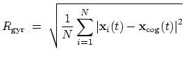 |
(41) |
This component must contain one atoms {...} block to
define the atom group, and returns a positive number, expressed in
Å.
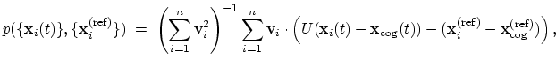
The block orientation {...} returns the
same optimal rotation used in the rmsd component to
superimpose the coordinates
onto a set of
reference coordinates
. Such
component returns a four dimensional vector
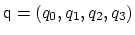 , with
 ; this quaternion
expresses the optimal rotation
; this quaternion
expresses the optimal rotation
 according to the formalism in
reference [18]. The quaternion
according to the formalism in
reference [18]. The quaternion
 can also be written as
 , where
  is the angle and
 the normalized axis of rotation; for example, a rotation
of 90
the normalized axis of rotation; for example, a rotation
of 90 around the axis should be expressed as
``(0.707, 0.0, 0.0, 0.707)''. The script
quaternion2rmatrix.tcl provides Tcl functions for converting
to and from a
around the axis should be expressed as
``(0.707, 0.0, 0.0, 0.707)''. The script
quaternion2rmatrix.tcl provides Tcl functions for converting
to and from a
 rotation matrix in a format suitable for
usage in VMD.
rotation matrix in a format suitable for
usage in VMD.
The component accepts all the options of rmsd:
atoms, refPositions, refPositionsFile and
refPositionsCol, in addition to:
- closestToQuaternion (orientation) Reference rotation
Acceptable Values: ``(q0, q1, q2, q3)'' quadruplet
Default Value: (1.0, 0.0, 0.0, 0.0) (``null'' rotation)
Description: Between the two equivalent quaternions
and
 , the closer to (1.0, 0.0, 0.0,
0.0) is chosen. This simplifies the visualization of the
colvar trajectory when samples values are a smaller subset of all
possible rotations. Note: this only affects the
output, never the dynamics.
, the closer to (1.0, 0.0, 0.0,
0.0) is chosen. This simplifies the visualization of the
colvar trajectory when samples values are a smaller subset of all
possible rotations. Note: this only affects the
output, never the dynamics.
Hint: stopping the rotation of a protein. To stop the
rotation of an elongated macromolecule in solution (and use an
anisotropic box to save water molecules), it is possible to define a
colvar with an orientation component, and restrain it throuh
the harmonic bias around the identity rotation, (1.0,
0.0, 0.0, 0.0). Only the overall orientation of the macromolecule
is affected, and not its internal degrees of freedom. The user
should also take care that the macromolecule is composed by a single
chain, or disable wrapAll otherwise.
The block
orientationAngle {...} accepts the same options as
rmsd and orientation (atoms,
refPositions, refPositionsFile and
refPositionsCol), but it returns instead the angle of
rotation  between the current and the reference positions.
This angle is expressed in degrees within the range
[0:180].
between the current and the reference positions.
This angle is expressed in degrees within the range
[0:180].
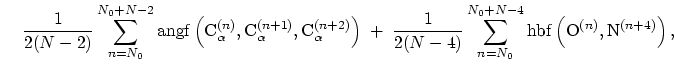
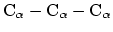
The block alpha {...} defines the
parameters to calculate the helical content of a segment of protein
residues. The -helical content across the  residues
 to
to  is calculated by the formula:
 |
|
|
(42) |
 |
|
|
|
where the score function for the
 angle is defined as:
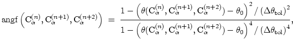 |
(43) |
and the score function for the
 hydrogen bond is defined through a hBond
colvar component on the same atoms. The options recognized within the
alpha {...} block are:
hydrogen bond is defined through a hBond
colvar component on the same atoms. The options recognized within the
alpha {...} block are:
This component returns positive values, always comprised between 0
(lowest -helical score) and 1 (highest -helical
score).
The block dihedralPC {...} defines the
parameters to calculate the projection of backbone dihedral angles within
a protein segment onto a dihedral principal component, following
the formalism of dihedral principal component analysis (dPCA) proposed by
Mu et al.[52] and documented in detail by Altis et
al.[2].
Given a peptide or protein segment of  residues, each with Ramachandran
angles
residues, each with Ramachandran
angles  and
and  , dPCA rests on a variance/covariance analysis
of the
, dPCA rests on a variance/covariance analysis
of the  variables
 . Note that angles
  and
and  have little impact on chain conformation, and are therefore discarded,
following the implementation of dPCA in the analysis software Carma.[26]
have little impact on chain conformation, and are therefore discarded,
following the implementation of dPCA in the analysis software Carma.[26]
For a given principal component (eigenvector) of coefficients
 ,
the projection of the current backbone conformation is:
,
the projection of the current backbone conformation is:
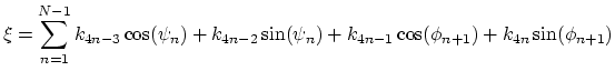 |
(44) |
dihedralPC expects the same parameters as the alpha
component for defining the relevant residues (residueRange
and psfSegID) in addition to the following:
Linear and polynomial combinations of components
Any set of components can be combined within a colvar, provided that
they return the same type of values (scalar, unit vector, vector, or
quaternion). By default, the colvar is the sum of its components.
Linear or polynomial combinations (following
equation (36)) can be obtained by setting the
following parameters, which are common to all components:
Example: To define the average of a colvar across
different parts of the system, simply define within the same colvar
block a series of components of the same type (applied to different
atom groups), and assign to each component a componentCoeff
of  .
.
Defining atom groups
Each component depends on one or more atom groups, which can be
defined by different methods in the configuration file. Each atom
group block is initiated by the name of the group itself within the
component block, followed by the instructions to the colvar module on
how to select the atoms involved. Here is an example configuration,
for an atom group called myatoms, which makes use of the most
common keywords:
# atom group definition
myatoms {
  # add atoms 1, 2 and 3 to this group (note: numbers start from 1)
  atomNumbers {
     1 2 3
  }
  # add all the atoms with occupancy 2 in the file atoms.pdb
  atomsFile             atoms.pdb
  atomsCol              O
  atomsColValue         2.0
  # add all the C-alphas within residues 11 to 20 of segments "PR1" and "PR2"
  psfSegID              PR1 PR2
  atomNameResidueRange  CA 11-20
  atomNameResidueRange  CA 11-20
}
For any atom group, the available options are:
- atomNumbers (atom group) List of atom numbers
Acceptable Values: space-separated list of positive integers
Description: This option adds to the group all the atoms whose numbers are in
the list. Atom numbering starts from 1.
- atomNumbersRange (atom group) Atoms within a number range
Acceptable Values: Starting number-Ending number
Description: This option adds to the group all the atoms whose numbers are
within the range specified. It can be used multiple times for the
same group. Atom numbering starts from 1. May be repeated.
- atomNameResidueRange (atom group) Named atoms within a range of residue numbers
Acceptable Values: Atom name Starting residue-Ending residue
Description: This option adds to the group all the atoms with the provided
name, within residues in the given range. May be repeated for as
many times as the values of psfSegID.
- psfSegID (atom group) PSF segment identifier
Acceptable Values: space-separated list of strings (max 4 characters)
Description: This option sets the PSF segment identifier for of
atomNameResidueRange. Multiple values can be provided,
which can correspond to different instances of
atomNameResidueRange, in the order of their occurrence.
This option is not needed when non-PSF topologies are used by
NAMD.
- atomsFile (atom group) PDB file name for atom selection
Acceptable Values: string
Description: This option selects atoms from the PDB file provided and adds them
to the group according to the value in the column
atomsCol. Note: the set of atoms PDB file
provided must match the topology.
- atomsCol (atom group) PDB column to use for the selection
Acceptable Values: X, Y, Z, O or B
Description: This option specifies which column in atomsFile is used
to determine the atoms to be included in the group.
- atomsColValue (atom group) Value in the PDB column
Acceptable Values: positive decimal
Description: If defined, this value in atomsCol identifies of
atomsFile which atoms are to be read; otherwise, all
atoms with a non-zero value will be read.
- dummyAtom (atom group) Dummy atom position (Å)
Acceptable Values: (x, y, z) triplet
Description: This option makes the group a virtual particle at a fixed position
in space. This is useful e.g. to make colvar components that
normally calculate functions of the group's center of mass use an
absolute reference position. If specified, disableForces
is also turned on, the center of mass position is (x, y,
z) and zero velocities and system forces are reported.
- centerReference (atom group) Ignore the translations of this group
Acceptable Values: boolean
Default Value: off
Description: If this option is on, the center of geometry of this
group is centered on a reference frame, determined either by
refPositions or refPositionsFile. This
transformation occurs before any colvar component has
access to the coordinates of the group: hence, only the recentered
coordinates are available to the colvars. Note:
the derivatives of the colvars with respect to the
translation are usually neglected (except by
rmsd and eigenvector).
- rotateReference (atom group) Ignore the rotations of this group
Acceptable Values: boolean
Default Value: off
Description: If this option is on, this group is rotated around its
center of geometry, to optimally superimpose to the positions
given by refPositions or refPositionsFile. This
is done before recentering the group, if centerReference
is also defined. The algorithm used is the same employed in the
orientation colvar component [18]. Forces
applied by the colvars to this group are rotated back to the
original frame prior being applied. Note: the
derivatives of the colvars with respect to the rotation are
usually neglected (except by rmsd and
eigenvector).
- refPositions (atom group) Reference positions (Å)
Acceptable Values: space-separated list of (x, y, z) triplets
Description: If either centerReference or rotateReference is
on, these coordinates are used to determine the center of
mass translation and the optimal rotation, respectively. In the
latter case, the list must also be of the same length as this atom
group.
- refPositionsFile (atom group) File with reference positions
Acceptable Values: UNIX filename
Description: If either centerReference or rotateReference is
on, the coordinates from this file are used to determine
the center of geometry translation and the optimal rotation between
them and the current coordinates of the group. This file can
either i) contain as many atoms as the group (in which case
all of the ATOM records are read) or ii) a larger
number of atoms. In the second case, coordinates will be selected either
according to flags in column refPositionsCol, or, if that
parameter is not specified, by index, using the list of atom indices
belonging to the atom group. In a typical application, a PDB file
containing both atom flags and reference coordinates is prepared, and
provided as both atomsFile and refPositionsFile,
while the flag column is passed to atomsCol and
refPositionsCol.
- refPositionsCol (atom group) Column to use in the PDB file
Acceptable Values: X, Y, Z, O or B
Description: Like atomsCol for atomsFile, indicates which
column to use to identify the atoms in refPositionsFile.
If not specified, atoms are selected by index, based on the
atom group definition.
- refPositionsColValue (atom group) Value in the PDB column
Acceptable Values: positive decimal
Description: Analogous to atomsColValue, but applied to
refPositionsCol.
- refPositionsGroup (atom group) Use an alternate group do perform roto-translational
fitting
Acceptable Values: Block refPositionsGroup { ... }
Default Value: This group itself
Description: If either centerReference or rotateReference is
defined, this keyword allows to define an additional atom group,
which is used instead of the current one to calculate the
translation or the rotation to the reference positions. For
example, it is possible to use all the backbone heavy atoms of a
protein to set the reference frame, but only involve a more
localized group in the colvar's definition.
- disableForces (atom group) Don't apply colvar forces to this group
Acceptable Values: boolean
Default Value: off
Description: If this option is on, all the forces applied from the
colvars to the atoms in this group are ignored. The applied
forces on each colvar are still written to the trajectory file, if
requested. In some cases it may be desirable to use this option
in order not to perturb the motion of certain atoms.
Note: when used, the biasing forces are not applied
uniformly: a non-zero net force or torque to the system is
generated, which may lead to undesired translations or rotations
of the system.
Note: to minimize the length of the NAMD standard output,
messages in the atom group's configuration are not echoed by default.
This can be overcome by the boolean keyword verboseOutput
within the group.
When defining the
atom groups for a collective variable, these guidelines should be
followed to avoid inconsistencies and performance losses:
- In simulations with periodic boundary conditions, NAMD maintains
the coordinates of all the atoms within a molecule contiguous to
each other (i.e. there are no spurious ``jumps'' in the molecular
bonds). The colvar module relies on this when calculating a group's
center of mass, but this condition may fail when the group spans
different molecules: in that case, writing the NAMD output files
wrapAll or wrapWater could produce wrong results
when a simulation run is continued from a previous one. There are
however cases in which wrapAll or wrapWater can be
safely applied:
- i)
- the group has only one atom;
- ii)
- it has all its atoms within the same molecule;
- iii)
- it is used by a colvar component which does not
access its center of mass and uses instead only interatomic
distances (coordNum, hBond, alpha);
- iv)
- it is used by a colvar component that ignores the
ill-defined Cartesian components of its center of mass (such as
the
 and
and  components of a membrane's center of mass by
distanceZ).
components of a membrane's center of mass by
distanceZ).
In the general case, the user should determine, according to which
type of calculation is being performed, whether wrapAll or
wrapWater can be enabled.
- Performance issues:
While NAMD spreads the calculation of most interaction terms
over many computational nodes, the colvars calculation is not
parallelized. This has two consequences: additional load on the
master node, where the colvar calculation is performed, and
additional communication between nodes.
NAMD's latency-tolerant design and dynamic load balancing
alleviate these factors; still, under some circumstances,
significant performance impact may be observed, especially in
the form of poor parallel scaling. To mitigate
this, as a general guideline, the size of atom groups
involved in colvar components should be kept small unless
necessary to capture the relevant degrees of freedom.
Statistical analysis of individual collective variables
When the global keyword analysis is defined in the
configuration file, calculations of statistical properties for
individual colvars can be performed. At the moment, several types of
time correlation functions, running averages and running standard
deviations are available.
- corrFunc (colvar) Calculate a time correlation function?
Acceptable Values: boolean
Default Value: off
Description: Whether or not a time correlaction function should be calculated
for this colvar.
- corrFuncWithColvar (colvar) Colvar name for the correlation function
Acceptable Values: string
Description: By default, the auto-correlation function (ACF) of this colvar,
 , is calculated. When this option is specified, the
correlation function is calculated instead with another colvar,
, is calculated. When this option is specified, the
correlation function is calculated instead with another colvar,
 , which must be of the same type (scalar, vector, or
quaternion) as .
, which must be of the same type (scalar, vector, or
quaternion) as .
- corrFuncType (colvar) Type of the correlation function
Acceptable Values: velocity, coordinate or
coordinate_p2
Default Value: velocity
Description: With coordinate or velocity, the correlation
function
 =
=
 is calculated between
the variables and , or their velocities.
is calculated between
the variables and , or their velocities.
 is the scalar product when calculated
between scalar or vector values, whereas for quaternions it is the
cosine between the two corresponding rotation axes. With
coordinate_p2, the second order Legendre polynomial,
is the scalar product when calculated
between scalar or vector values, whereas for quaternions it is the
cosine between the two corresponding rotation axes. With
coordinate_p2, the second order Legendre polynomial,
 , is used instead of the cosine.
- corrFuncNormalize (colvar) Normalize the time correlation function?
Acceptable Values: boolean
Default Value: on
Description: If enabled, the value of the correlation function at  = 0
is normalized to 1; otherwise, it equals to
= 0
is normalized to 1; otherwise, it equals to
 .
.
- corrFuncLength (colvar) Length of the time correlation function
Acceptable Values: positive integer
Default Value: 1000
Description: Length (in number of points) of the time correlation function.
- corrFuncStride (colvar) Stride of the time correlation function
Acceptable Values: positive integer
Default Value: 1
Description: Number of steps between two values of the time correlation function.
- corrFuncOffset (colvar) Offset of the time correlation function
Acceptable Values: positive integer
Default Value: 0
Description: The starting time (in number of steps) of the time correlation
function (default: = 0). Note: the value at = 0 is always
used for the normalization.
- corrFuncOutputFile (colvar) Output file for the time correlation function
Acceptable Values: UNIX filename
Default Value: name.corrfunc.dat
Description: The time correlation function is saved in this file.
- runAve (colvar) Calculate the running average and standard deviation
Acceptable Values: boolean
Default Value: off
Description: Whether or not the running average and standard deviation should
be calculated for this colvar.
- runAveLength (colvar) Length of the running average window
Acceptable Values: positive integer
Default Value: 1000
Description: Length (in number of points) of the running average window.
- runAveStride (colvar) Stride of the running average window values
Acceptable Values: positive integer
Default Value: 1
Description: Number of steps between two values within the running average window.
- runAveOutputFile (colvar) Output file for the running average and standard deviation
Acceptable Values: UNIX filename
Default Value: name.runave.dat
Description: The running average and standard deviation are saved in this file.
Next: Biasing and analysis methods
Up: Collective Variable-based Calculations1
Previous: General parameters and input/output
Contents
Index
http://www.ks.uiuc.edu/Research/namd/