


Next: Modeling amino acid insertions
Up: Rosetta/MDFF Tutorial
Previous: Required software
Contents
Subsections
Folding protein termini using ModelMaker
Here, we predict a structural model for the truncated C-terminal tail from amino acid 217 to 306 of chain B of 4OCM. Create a folder named terminus for this section and navigate to it. Sample input and output files are provided
in the 3.terminus folder in the tutorial folder.
First you need to obtain a template structure which should be completed by modeling the structurally unresolved segments. In this tutorial we complete Rpn11, the deubiquitilyation subunit of the 26S proteasome. As template for modeling, we use chain B of PDB structure 4OCM. Go to the Protein Data Bank (PDB, http://www.rcsb.org/pdb/home/home.do) and download the PDB structure with the PDB-ID 4OCM. Alternatively you can download the PDB structure directly through VMD by going to File  New Molecule, type 4OCM in the Filename box and click the Load button. The PDB structure 4OCM contains two Rpn8/Rpn11 dimers in the unit cell. For now we only need one Rpn11, so we use chain B. In order to create a PDB file containing only chain B run the following command in the TK console (Extensions Tk Console):
[atomselect top "chain B and protein"] writepdb rpn11_yeast_4ocm.pdb
Structure prediction
In order to use ModelMaker for structure prediction you first need to modify the configuration file.
- 1
- Preparing the configuration file:
Copy the prepared
configuration file fold_rpn11_terminus.tcl from the tutorial files to your terminus folder, open it in a text editor and change the following
variables to fit your workstation configuration.
Table 1:
Default configuration variables
| variable |
description |
| packagePath |
path of the ModelMaker plugin files |
| vmdexe |
path of your vmd executable |
| gnuplotexe |
path of your gnuplot executable |
| rosettapath |
directory path containing the Rosetta binaries |
| rosettaDBpath |
Rosetta database path |
| platform |
"linuxgccrelease" or "macosclangrelease" |
|
- 2
- Obtaining the target amino acid residue sequence:
As we are only going to fold the C-terminus of Rpn11, we will discard the missing N-terminus in our following
procedures. Go to the uniprot website (http://www.uniprot.org)
and download the fasta sequence of Rpn11 in yeast (UniprotID: P43588).
Create a folder called input.
With a text editor, remove the first 22 amino acids
from the sequence and save the file in the input folder as rpn11_yeast_23-306.fasta.
To facilitate the sub-sequence extraction, a Python script subrange.py is provided in the scripts folder, that you can
use to get the amino acid codes for a given range. Simply copy the script to your working directory and make the following changes:
- line 3: start defines the start of the sequence
- line 4: end defines the end of the sequence
- line 6: name defines the input name of the given fasta sequence
Running
python subrange.py
creates a file <name>_<start>-<end>.fasta from the input fasta sequence.
- 3
- Generating the fragment file library:
Use the Robetta server to generate two library files containing internal coordinates for the target sequence structure. The server performs a homolgy search algorithm in the PDB Data Bank based on a running window of 3 and 9 amino acid length and produce two files (3mer and 9mer) presenting the best 200 results for each window. To do so, go to http://www.robetta.org
and set an academic user account. Submit the target sequence rpn11_yeast_23-306.fasta to the Fragment file server and as soon as the search is finished you will receive an email with a link to download the results. Save the 3mer and 9mer files as rpn11_yeast_23-306.frag3 and rpn11_yeast_23-306.frag9 in your input folder.
- 4
- Building one complete model for the target amino acid sequence:
Create a full_length_model folder and copy the file rpn11_yeast_4ocm.pdb to it.
Furthermore, copy the file run_full_length_model.sh from the tutorial files to your full_length_model folder.
Make the following changes in run_full_length_model.sh:
- line 9: rosetta=/path/to/rosetta/bin
indicates the path to your Rosetta binary directory.
- line 11: platform="linuxgccrelease"
supplies the platform Rosetta has been built on, thus either
platform="linuxgccrelease" or
platform="macosclangrelease" is accepted.
Run run_full_length_model.sh to generate a complete template model. Afterwards, rename the output file rpn11_yeast_4ocm.pdb_full_length.pdb to rpn11_yeast_23-306_complete.pdb.
./run_full_length_model.sh
mv rpn11_yeast_4ocm.pdb_full_length.pdb rpn11_yeast_23-306_complete.pdb
Rosetta's full length modell application yields PDB files that do not keep the original amino acid numbering. To keep it, copy the script renumber.tcl from
the scripts folder to the full_length_model folder. In the mols list, you can specify the file name of the input PDB file, in this case, the line should look like:
set mols [list rpn11_yeast_23-306_complete.pdb]
In the next line, you can set the newstart varible to 23, so that the output PDB file starts its numbering from 23, as in the fasta file. Run
vmd -dispdev text -e renumber.tcl
to get the output file rpn11_yeast_23-306_complete-numb.pdb, then replace the old file with the new one:
mv rpn11_yeast_23-306_complete-numb.pdb rpn11_yeast_23-306_complete.pdb.
- 5
- Running Rosetta from VMD:
Now that we have prepared all necessary input files, we can complete the configuration file to finally run Rosetta from VMD
to predict the C-terminal structure of Rpn11.
The recommendation from the literature is to predict between 5,000 and 20,000 modelss. In our test case we predict only 100 structures for demonstration purpose. We use RosettaScripts with a Brokered Environment and execute the classic Rosetta de novo protocol upon it. The ModelMaker plugin can handle input file generation for Rosetta automatically, so we just need to add a few lines
to fold_rpn11_terminus.tcl.
- line 14: set nstruct 100
creates a variable that is later on passed to Rosetta and indicates the number
of structures to generate.
- line 15: set bestN 25
shows the number of highest scored structures that should be taken into account for analysis.
- line 18: set tempPath [pwd]/full_length_model
points to the path containing the full length Rpn11 model, created in the step before.
- line 20: set tempdir [pwd]/full_length_model
points to the path containing the PDB file for alignment in the analysis step. If you have an alternative PDB file you want to align the predicted models to, you can specify it by setting tempdir. In our test case, we simply use the full length model for alignment as well.
- line 22: set comps [list [list ss 196 284 "A"]]
sets a list to define analysis tasks for the predicted structures. The ModelMaker packages can take a list of several analysis tasks. Here, we only define a secondary structure
analysis task, that scans the amino acids 196 to 284 of chain A for the average secondary structure.
The secondary structure analysis task is
configured by the list in $comps, where the single elements stand for:
[list ss  start residue ID
 end residue ID chain]
- line 25: start_rosetta_abinitio ...
starts a Rosetta structure prediction task with the given arguments in Tab. 2.
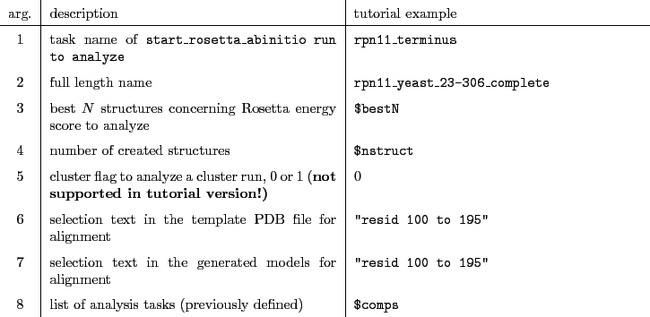
- line 27: analyze_abinitio ...
starts the analysis procedure. The argument configuration is explained in Tab. 3. This command automatically calls Rosetta energy scoring, aligns the best  ($bestN) structures and performs the analysis tasks defined in $comps.
Execute the configuration file in VMD text mode and wait for the tasks to finish. Depending on the number
of structures to generate, this may take a while.
vmd -dispdev text -e fold_rpn11_terminus.tcl
If no error occurs, go to the folder called rosetta_output_rpn11_terminus containing the results
of your run.
Table 2:
Rosetta ab initio procedure arguments
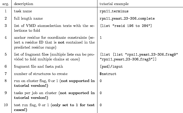 |
Table 3:
Rosetta ab initio analysis procedure arguments
 |
Interactive fitting to a cryo-EM density with iMDFF and QwikMD
Create a new folder named mdff in your working directory.
- 1
- Aligning the predicted model with the cryo-EM density map:
In order to perform interartive molecular dynamics flexible fitting you first need to place the modeled structure in the right position inside the density map. Download the cryo-EM density map of the 26S proteasome (EMDB-ID 2594) from the electron microscopy database (http://www.ebi.ac.uk/pdbe/emdb/): emd_2594.map. In this special case there exist already a near-atomic structural model (PDB-ID 4CR2) for this map. Download the structure with the PDB-ID 4CR2 from the PDB (http://www.rcsb.org/pdb/home/home.do). Use align_segments.tcl to align the output structure from the structure prediction (ss_average_100.pdb) to chain V of 4CR2.pdb in order to get ss_average_100_aligned.pdb.
- 2
- Generating a density map file for MDFF:
In order to generate a readable density map file for MDFF the file emd_2594.map first needs to be renamed to emd_2594.ccp4 and then run the command in your terminal (The script is contained in the scripts folder):
vmd -dispdev text -e get_density.tcl
which will excecute
mdff griddx -i emdb_2594.ccp4 -o emdb_2594_potential.dx
mdff griddx -i emdb_2594_potential.dx -o emdb_2594_density.dx
to obtain the density file emdb_2594_density.dx, which can be read by MDFF.
- 3
- Crop the density:
In order to crop the density to the area of interest, which is here around the predicted structural model of Rpn11, run crop_density.tcl.
vmd -dispdev text -e crop_density.tcl
The script generates the density file rpn11_model_5_2594_density.dx, which contains the density of emd_2594_density.dx within a cutoff of  around .
- 4
- Fitting the modeled part to the cryo EM density:
We are going to use the VMD plugin QwikMD to setup the interactive MDFF run as it automatically generates
all the required input files and structures.
- Run VMD and open the QwikMD plugin (Extensions Simulation QwikMD).
- Browse to the average secondary structure PDB file ss_average_25.pdb located at ./rosetta_output_rpn11_terminus/analysis/ss_196_284/ and load it into QwikMD.
- Click on Structure Manipulation and ignore occurring errors.
- On top, navigate to the Advanced Run tab and select the MDFF tab.
- In the Protocol dropdown menu,
adjust Fixed to "resid 1 to 195" and select "same fragment as protein" for Sec. Structure, Chirality and Cispeptide restraints.
- Click on Prepare and give your QwikMD file the name rpn11_terminus_mdff when prompted.
QwikMD automatically generates the necessary PSF file and restraint files and redirects you to the MDFF graphical user interface.
- Open the MDFF files dropdown and add the cropped density
rpn11_model_5_2594_density.dx
- To improve performance, you can adjust the number of CPU cores NAMD should use for the MDFF run by changing the value
for Processors in the IMD parameters dropdown.
- Click on the IMDFF Connect tab on top of the MDFF GUI and open the Cross Correlation Analysis dropdown.
- Check Calculate real-time Cross Correlation, set Experimental Density (Mol ID) to the Mol ID of the loaded density (you can obtain the ID from the first column of the VMD Main menu) and set the Map Resolution to
 .
.
- Click on Submit and Connect to start the simulation and interact with it through the VMD window.
Hint: If you have problems moving the structure to the correct positions, load the final Rpn11 structure rpn11_yeast.pdb from the tutorial folder into VMD while performing iMDFF.
In the first step drag the predicted structure to the density apply forces (Mouse Forces Atom) by clicking on an atom. In this step a grid spacing of 0.3 should be applied. For detailed instructions on the usage of the MDFF GUI and interactive fitting see the MDFF tutorial and the Youtube tutorial https://www.youtube.com/watch?v=-KJiH_WF65s. As soon as the predicted segment fits the density a second MDFF run with a grid spacing of 0.6 can be performed.
Hint: Use cartoon representation for the protein with different coloring for the fixed and flexible segments. Represent the density as solid surface with white color and transparent material. Use the CPK representation for the backbone atoms of the flexible segment and apply only forces to these backbone atoms.
Next: Modeling amino acid insertions
Up: Rosetta/MDFF Tutorial
Previous: Required software
Contents
www.ks.uiuc.edu/Training/Tutorials