Stretching Deca-Alanine: Analysis

Next: PMF calculation Up: Stretching Deca-Alanine Previous: Viewing SMD trajectories within VMD

Analysis of the SMD trajectory

We will be using MATLAB from now on. Start MATLAB:

tbss> matlab

MATLAB commands should be entered in Command Window. We will use the tag >> to indicate MATLAB commands.

Load the Tcl output file generated by your SMD simulation and store it to a matrix mytraj:

>> mytraj = load('da_smd_tcl.out');

Print the content of mytraj on the screen.

>> mytraj

You should see a matrix containing three columns.
First column: time (ps)
Second column: extension, or the end-to-end distance (Å)
Third column: applied force (kcal/mol/Å)

We use the following units: ps for time, Å for distance, kcal/mol for energy.

Assign columns of mytraj to separate arrays:

>> t = mytraj(:,1);
>> z = mytraj(:,2);
>> f = mytraj(:,3);

Define parameters, v (pulling velocity) and dt (time step of the data):

>> v = 1;
>> dt = 0.1;

Recall that one end of the molecule was constrained to the origin and the other end was constrained to a moving point. The distance between the two constraints was changed from 13 Å to 33 Å with the constant velocity v. Define an array c representing the distance between the two constraint points at each time step:

>> c = (13:v*dt:33)';

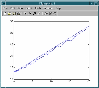
Plot the z-t and c-t curves:

>> figure; hold on
>> plot(t,z)
>> plot(t,c)

Q: The extension z generally lags behind c, the distance between the two constraints. How big is the lag in this case? What would you do if you want to reduce the lag further?

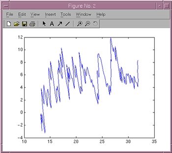
Plot the force-extension curve:
>> figure; plot(z,f)
Q: Is the force generally positive or negative? Why?

The work done on the system during the pulling simulation is

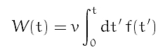
where v is the pulling velocity.

Calculate the work W by numerical integration:

>> W = v*dt*cumsum(f);

If a pulling simulation is performed very slowly, then the process is reversible. The work done during such a reversible pulling is equal to the free energy difference of the system between initial and final states. Thus, a reversible work curve can be considered as an exact PMF. For our system, the reversible pulling speed turns out to be about 0.0001 Å/ps (10000 times slower than the one you used).

The exact PMF obtained from a reversible pullings is stored as a variable Fexact in a file da.mat. Load it:
>> load da.mat Fexact
Plot W-c in blue together with Fexact in red:
>> figure; hold on >> plot(c,W,'b') >> plot(Fexact(:,1),Fexact(:,2),'r')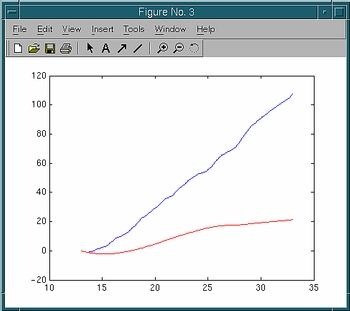

Q: How do they compare? What is the origin of the difference?

Quit MATLAB:

>> quit

Next: PMF calculation Up: Stretching Deca-Alanine Previous: Viewing SMD trajectories within VMD