Stretching Deca-Alanine: PMF

Up: Stretching Deca-Alanine Previous: Analysis of the SMD trajectory

PMF calculation

The trajectory you have generated in this session is actually not practical for the PMF calculation because the pulling speed was too high. Besides, you need multiple trajectories to use Jarzynski's equality. Therefore, you will use pre-generated trajectories.

Start MATLAB:

tbss> matlab

Ten trajectories obtained from SMD simulations with a pulling speed of 0.01 Å/ps are stored in da.mat. This pulling speed is 100 times slower than the one you used, but still 100 times faster than the reversible speed. Load the trajectories as well as the exact PMF:

>> load da.mat t z f Fexact

The array t contains time steps of the data. z and f are matrices of 10 columns, with each column representing the extension and the applied force for each trajectory, respectively.

Plot the extension-time curve:

>> figure; plot(t,z)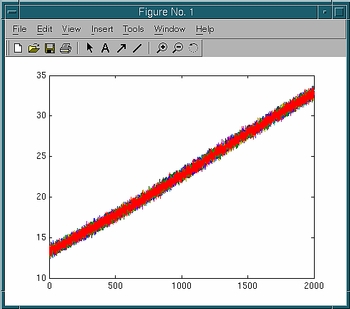

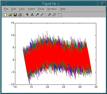
And plot the force-extension curve:
>> figure; plot(z,f)
In each figure window, you should see ten overlapping curves, with each curve corresponding to a trajectory.

Define parameters: dt, time step; v, pulling speed; T, temperature (including Boltzmann's constant).
>> dt = 0.1; >> v = 0.01; >> T = 0.6;
Define an array c representing the distance between the two constraint points at each time step:
>> c = (13:v*dt:33)';
Calculate work for each trajectory. The following single command will do:
>> W = v*dt*cumsum(f,1);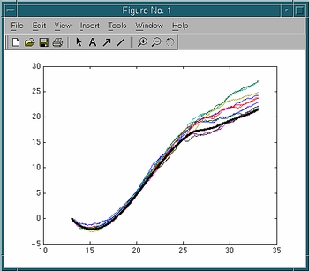

Plot W vs. c together with the exact PMF:

>> figure; hold on
>> plot(c,W)
>> plot(Fexact(:,1),Fexact(:,2),'k','linewidth',3);

You should see ten work curves and one curve for the exact PMF. Thick black line is the exact PMF.

Q: Work done to the system should be on average higher than the PMF. Are all the work curves higher than the PMF, or do you also see some work curves lower than the PMF?

Let's now employ Jarzynski's equality:

The right-hand side can be expanded in terms of so-called cumulants:

where the cumulants up to the second order are shown.

Estimate the PMF according to three different formulae: the original formula (exponential average), the first order cumulant expansion formula (average work), and the second order cumulant expansion formula.

>> Fexp = -T*log(mean(exp(-W/T),2));
>> F1 = mean(W,2);
>> F2 = mean(W,2) - 1/2/T*(mean(W.^2,2)-mean(W,2).^2);

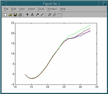
Plot the three estimates for the PMF together with the exact PMF. Plot the exact PMF Fexact in red, the average work (or the first order cumulant expansion) F1 in green, the second order cumulant expansion F2 in blue, and the exponential average Fexp in black:

>> figure; hold on
>> plot(Fexact(:,1),Fexact(:,2),'r');
>> plot(c,F1,'g');
>> plot(c,F2,'b');
>> plot(c,Fexp,'k');

Q: Which estimate is the closest to the exact PMF? Does it make sense to you in view of what you learnt in the lecture?

Quit MATLAB:

>> quit

For more information on the PMF calculation from SMD simulations, see the paper included:

tbss> acroread paper.pdf &

Up: Stretching Deca-Alanine Previous: Analysis of the SMD trajectory