Free energy differences can be obtained through four different routes: (i) probability densities, (ii) free energy perturbation, (iii) thermodynamic integration, or (iv) nonequilibrium work approaches [16]. Within NAMD, alchemical transformations are modeled following the second and the third routes, both of which rely upon the use of a general extent parameter often referred to as the coupling parameter [8,45,36,37] for the description of chemical changes in the molecular systems between the reference and the target states.
In a typical alchemical transformation setup involving the alteration of one
chemical species into an alternate one in the course of the simulation, the
atoms in the molecular topology can be classified into three groups, (i) a
group of atoms that do not change during the simulation -- e.g. the
environment, (ii) the atoms describing the reference state, ![]() , of the
system, and (iii) the atoms that correspond to the target state,
, of the
system, and (iii) the atoms that correspond to the target state, ![]() , at the
end of the alchemical transformation. The atoms representative of state
, at the
end of the alchemical transformation. The atoms representative of state ![]() should never interact with those of state
should never interact with those of state ![]() throughout the MD
simulation. Such a setup, in which atoms of both the initial and the final
states of the system are present in the molecular topology file -- i.e. the
psf file -- is characteristic of the so-called ``dual topology''
paradigm [23,54,3]. The hybrid Hamiltonian
of the system is a function of the general extent parameter,
throughout the MD
simulation. Such a setup, in which atoms of both the initial and the final
states of the system are present in the molecular topology file -- i.e. the
psf file -- is characteristic of the so-called ``dual topology''
paradigm [23,54,3]. The hybrid Hamiltonian
of the system is a function of the general extent parameter, ![]() ,
which connects smoothly state
,
which connects smoothly state ![]() to state
to state ![]() . In the simplest case, such a
connection may be achieved by linear combination of the corresponding Hamiltonians:
. In the simplest case, such a
connection may be achieved by linear combination of the corresponding Hamiltonians:
where
![]() describes the interaction of
the group of atoms representative of the reference state,
describes the interaction of
the group of atoms representative of the reference state, ![]() , with the rest of
the system.
, with the rest of
the system.
![]() characterizes the interaction of
the target topology,
characterizes the interaction of
the target topology, ![]() , with the rest of the system.
, with the rest of the system.
![]() is the Hamiltonian describing those atoms that do not undergo any
transformation during the MD simulation.
is the Hamiltonian describing those atoms that do not undergo any
transformation during the MD simulation.
For instance, in the point mutation of an alanine side chain into that of
glycine, by means of a free energy calculation -- either free energy
perturbation or thermodynamic integration, the topology of both the methyl
group of alanine and the hydrogen borne by the C![]() in glycine co-exist
throughout the simulation (see Figure 7), yet without actually
seeing each other.
in glycine co-exist
throughout the simulation (see Figure 7), yet without actually
seeing each other.
![\includegraphics[width=12.5cm]{figures/dual_top}](img421.png) |
The energy and forces are defined as a function of ![]() , in such a fashion
that the interaction of the methyl group of alanine with the rest of the
protein is effective at the beginning of the simulation, i.e.
, in such a fashion
that the interaction of the methyl group of alanine with the rest of the
protein is effective at the beginning of the simulation, i.e. ![]() = 0,
while the glycine C
= 0,
while the glycine C![]() hydrogen atom does not interact with the rest of
the protein, and vice versa at the end of the simulation, i.e.
hydrogen atom does not interact with the rest of
the protein, and vice versa at the end of the simulation, i.e. ![]() = 1. For intermediate values of
= 1. For intermediate values of ![]() , both the alanine and the glycine
side chains participate in nonbonded interactions with the rest of the protein,
scaled on the basis of the current value of
, both the alanine and the glycine
side chains participate in nonbonded interactions with the rest of the protein,
scaled on the basis of the current value of ![]() . It should be clearly
understood that these side chains never interact with each other.
. It should be clearly
understood that these side chains never interact with each other.
It is noteworthy that end points of alchemical transformations carried out in the framework of the dual-topology paradigm have been shown to be conducive to
numerical instabilities from molecular dynamics simulations, often coined as ``end-point
catastrophes''. These scenarios are prone to occur when ![]() becomes close
to 0 or 1, and incoming atoms instantly appear where other particles are
already present, which results in a virtually infinite potential as the
interatomic distance tends towards 0. Such ``end-point catastrophes'' can be
profitably circumvented by introducing a so-called soft-core
potential [7,44], aimed at a gradual scaling of the short-range
nonbonded interactions of incoming atoms with their environment, as shown in Equation 58.
What is really being modified is the value of a coupling parameter (
becomes close
to 0 or 1, and incoming atoms instantly appear where other particles are
already present, which results in a virtually infinite potential as the
interatomic distance tends towards 0. Such ``end-point catastrophes'' can be
profitably circumvented by introducing a so-called soft-core
potential [7,44], aimed at a gradual scaling of the short-range
nonbonded interactions of incoming atoms with their environment, as shown in Equation 58.
What is really being modified is the value of a coupling parameter (
![]() or
or
![]() ) that
scales the interactions -- i.e., if set to 0, the latter are off; if set to 1,
they are on -- in lieu of the actual value of
) that
scales the interactions -- i.e., if set to 0, the latter are off; if set to 1,
they are on -- in lieu of the actual value of ![]() provided by the user.
provided by the user.
It is also worth noting that the free energy calculation does not alter intermolecular bonded potentials, e.g. bond stretch, valence angle deformation and torsions, in the course of the simulation. In calculations targeted at the estimation of free energy differences between two states characterized by distinct environments -- e.g. a ligand, bound to a protein in the first simulation, and solvated in water, in the second -- as is the case for most free energy calculations that make use of a thermodynamic cycle, perturbation of intramolecular terms may, by and large, be safely avoided [10]. This property is controlled by the alchDecouple keyword described in
Within the FEP framework
[8,15,16,24,38,45,66,69,74],
the free energy difference between two
alternate states, ![]() and
and ![]() , is expressed by:
, is expressed by:
Here,
![]() , where
, where ![]() is the Boltzmann
constant,
is the Boltzmann
constant, ![]() is the temperature.
is the temperature.
![]() and
and
![]() are the Hamiltonians describing states
are the Hamiltonians describing states ![]() and
and ![]() ,
respectively.
,
respectively.
![]() denotes an ensemble average
over configurations representative of the initial, reference state,
denotes an ensemble average
over configurations representative of the initial, reference state, ![]() .
.
![\includegraphics[width=4cm]{figures/overlap1}](img430.png) (a)
(a)
![\includegraphics[width=4cm]{figures/overlap2}](img431.png) (b)
(b)
![\includegraphics[width=4cm]{figures/overlap3}](img432.png) (c)
(c) |
Convergence of equation (59) implies that low-energy configurations
of the target state, ![]() , are also configurations of the reference state,
, are also configurations of the reference state, ![]() ,
thus resulting in an appropriate overlap of the corresponding ensembles -- see
Figure 8. Transformation between the two
thermodynamic states is replaced by a series of transformations between
non-physical, intermediate states along a well-delineated pathway that
connects
,
thus resulting in an appropriate overlap of the corresponding ensembles -- see
Figure 8. Transformation between the two
thermodynamic states is replaced by a series of transformations between
non-physical, intermediate states along a well-delineated pathway that
connects ![]() to
to ![]() . This pathway is characterized by the general extent
parameter [8,36,37,45],
. This pathway is characterized by the general extent
parameter [8,36,37,45], ![]() , that
makes the Hamiltonian and, hence, the free energy, a continuous function of
this parameter between
, that
makes the Hamiltonian and, hence, the free energy, a continuous function of
this parameter between ![]() and
and ![]() :
:
Here, ![]() stands for the number of intermediate stages, or ``windows''
between the initial and the final states -- see Figure 8.
stands for the number of intermediate stages, or ``windows''
between the initial and the final states -- see Figure 8.
An alternative to the perturbation formula for free energy calculation is Thermodynamic Integration (TI). With the TI method, the free energy is given as [37,65,22]:
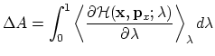 |
(60) |
In the multi-configuration thermodynamic integration approach
[65] implemented in NAMD,
![]() , the ensemble average
of the derivative of the internal energy with respect to
, the ensemble average
of the derivative of the internal energy with respect to ![]() , is
collected for a series of discrete
, is
collected for a series of discrete ![]() values and written to tiOutFile. These values are analyzed by the separately distributed script
NAMD_ti.pl, which performs the integration of individual energy
components and reports back the total
values and written to tiOutFile. These values are analyzed by the separately distributed script
NAMD_ti.pl, which performs the integration of individual energy
components and reports back the total ![]() values for the transformation.
values for the transformation.
![$\displaystyle V_\mathrm{NB}(r_{ij}) = \lambda_\mathrm{LJ} \varepsilon_{ij} \lef...
...ht)^{\!\!3} \right] + \lambda_\mathrm{elec} \frac{q_iq_j}{\varepsilon_1 r_{ij}}$](img424.png)
![$\displaystyle \Delta A_{a \rightarrow b} = -\frac{1}{\beta} \ \ln \left\langle ...
...}, {\bf p}_x) - {\cal H}_a({\bf x}, {\bf p}_x) \right] \right\} \right\rangle_a$](img425.png)
![$\displaystyle \Delta A_{a \rightarrow b} = -\frac{1}{\beta} \ \sum_{i = 1}^N \l...
...+1}) - {\cal H}({\bf x}, {\bf p}_x; \lambda_i) \right] \right\} \right\rangle_i$](img433.png)