Visualizing Global Datasets with Explorer 2.0

James C. Phillips

Paul J. Morin and David A. Yuen

Abstract

I. Introduction

II. The WorldMap Module

The CIA Map Directory parameter should be set to the directory in which the CIA and plate boundary maps may be found. The CIA maps are included with this module or are available by anonymous ftp from sepftp.stanford.edu in /pub/World_Map. The compressed version found there will untar into a map directory with subdirectories named africa.Map, asia.Map, europe.Map, namer.Map, and samer.Map. The original database (not the compressed version used here) is available from the U.S. Government and is in the public domain. The USGS_plates.txt file included with this module should be added to the map directory if you need plate boundary maps. The maps consume about 13 megabytes of disk space.

The Precision parameter should be set to the size, in seconds, of the largest feature which the decimation routine will eliminate. Usually this should be no higher that 3600 seconds (1 degree). A setting of 1 second will include all features since raw map coordinates are in integer numbers of seconds. Most features on the map appear to be on the order of thirty seconds. The decimation algorithm operates by combining as many line segments smaller than precision as possible such that their total vector length is still less than Precision into a single line segment. This will tend to eliminate features smaller than Precision and small islands may be reduced to a segment of zero length.

Remember that the map files are greatly compressed and when read into memory the map will be much larger. It is best to start at lower resolution with fewer features and build up than to attempt to read in the entire map at full resolution. One must use less resolution when looking at large areas and higher resolution when zooming in. This will also improve the drawing time for the map.

The Min/Max Latitude/Longitude parameters control the region of the earth to be mapped and are in degrees. Latitudes may take on any value and may span more than 360 degrees. Longitudes are limited to the range -90 to 90.

The option menus should be self explanatory with only a couple clarifications. The International and National menus refer to political boundaries. National boundaries only exist for the U.S. states and Canadian provinces. Boundaries which are also coastlines or rivers are not included in the boundary files. Thus, in order to see the outline of Minnesota, it is necessary to turn on Major Coastlines, Major Rivers, Definite International, and Definite National as in figure 19.

Most of the option menus (see exceptions below) operate on the principle that if you want, for example, Minor Rivers, you also want Major Rivers. Therefore selecting a feature on an option menu implies selecting all features above it on the menu as well. Of course some options, such as Plates, are simply all or none.

The Reefs, etc. and Ice menus are the exception to the above. Due to the limited number of input ports allowed by explorer, it was necessary to combine features in these menus. Thus the options are none, one, the other, or both.

The Parallels and Meridians menus place grid lines on the map, spaced as indicated. The lines consist of 1 degree segments and will therefore curve when used with the Projector module.

The output pyramid follows the finite element convention and is suitable for feeding into PyrToGeom. The coordinates are curvilinear and of the form (longitude, latitude, 0.0). There is a single data variable which is set to a number from 0 to 99 depending on the particular feature that is represented. When a colormap is used with PyrToGeom, this data allows each feature to have different color. See Appendix I for details.

III. The Projector Module

The Projector module has input ports for several pyramids and lattices and modifies the coordinates of its input to produce a projection. The first pyramid is designated the map and its z coordinate may be transformed to place the map above or below the data.

All lattices (including the base lattices of the pyramids) are assumed to have three coordinate variables. Any lattice with uniform or perimeter coordinates is also assumed to be three dimensional. All coordinates are assumed to represent longitude, latitude, and altitude (depths should be negative values). Longitude and latitude should be in degrees. Latitude may take on any value but the Base Longitude parameter (see below) should be set to compensate.

The Globe Radius parameter is required and should contain the radius of the earth in the same units as the altitudes in the data set. This parameter is used in all map projections to provide proper scaling of longitude and latitude.

The Map z parameter sets the amount the 1st. pyramid (the Map) will be shifted in the positive z direction. This allows the map (which is usually at z=0) to be placed, for example, above air masses or below seismic data.

The Projection option menu is used to select the particular map projection to be applied. These projections make use of some or all of the Base Longitude, Base Latitude, 1st. Standard Parallel, and 2nd. Standard Parallel dials so these will be discussed first.

The Base Longitude and Base Latitude parameters indicate the point on the globe which will be the center of the map. This is important because this is usually the area with the least distortion. The Base Longitude parameter may take on any value, but should be in the same range as the data. The Base Latitude parameter is limited to the range [-90,90].

The 1st. and 2nd. Standard Parallels are used by the conic projections to indicate the intersection of the cone with the earth. These parameters should be chosen to border the area of interest and the 1st. should be greater than or equal to the 2nd. If they are equal, the cone will only touch the earth and not penetrate it.

The implemented projections are listed below along with a brief explanation of their properties, utility, and parameters. Projections are classified according to their properties. A projection may be conformal, preserving the shapes of structures while distorting their scale, equivalent, preserving the area of structures, or equidistant, preserving distances in one or more directions. A Projection may also be azimuthal, based on some projection of the globe onto a plane tangent at one point, cylindrical, based on the projection of the globe onto a cylinder tangent (usually) at the equator, or conic, based on the projection of the globe onto a cone which intersects the globe at one or two standard parallels.

Available Projections

Cartesian (Fig 1)

Parameters: Base Long., Base Lat.
Properties: None
Longitude and Latitude map directly to x and y except that they are scaled to make equatorial and meridian distances correct in proportion to altitudes. This projection is seldom seen on maps, is considered cylindrical, and preserves no particular quality. The parameters only set the center of the map.

Mercator Cylindrical (Figs 2, 15, 16, & 18)

Parameters: Base Long., Base Lat.
Properties: Conformal
This is the standard Mercator projection. It is a cylindrical conformal projection. This projection goes to infinity as latitude approaches the poles, therefore such data should be cropped. The parameters only set the center of the map.

Lambert Cylindrical (Fig 3)

Parameters: Base Long., Base Lat.
Properties: Equivalent
This is an equivalent projection. Structures at the poles become flat in this projection. The parameters only set the center of the map.

Gnomonic Azimuthal (Fig 4)

Parameters: Base Long., Base Lat.
Properties: None
Projection is made from a perspective point at the center of the globe onto a plane which is tangent to the globe at (Base Longitude, Base Latitude). As with all azimuthal projections, great circles on the globe passing through the tangent point appear as straight lines radiating from it. This is the simplest azimuthal projection but has no special properties. Care should be taken in cropping data to avoid points which appear on the other side of the world from the tangent point, as this will produce undesirable results.

Stereographic Azimuthal (Fig 5)

Parameters: Base Long., Base Lat.
Properties: Conformal
Projection is made as above but from a perspective point on the surface of the globe exactly opposite the tangent point. This projection has the added property of being conformal. As above, all data points should be on the same side of the globe as the tangent point.

Orthonormal Azimuthal (Fig 6)

Parameters: Base Long., Base Lat.
Properties: None
Projection is made onto a plane as above from a point at infinity. This projection gives the effect of looking a a globe, but the projection is flat. Data points should be on the same side of the globe as the tangent point. To achieve the effect of looking at a globe, the actual Globe projection is recommended.

Postel Azimuthal (Fig 7)

Parameters: Base Long., Base Lat.
Properties: Equidistant
Also known as the azimuthal equidistant projection, this is useful for determining distances from a given origin. The distance from the point (Base Longitude, Base Latitude) to any other point on the map will be equal to that actual distance on the surface of the earth.

Lambert Azimuthal (Fig 8)

Parameters: Base Long., Base Lat.
Properties: Equivalent
Lambert's azimuthal equivalent projection. There is no distortion of area and the minimal distortion of shape occurs at the base point.

Lambert Conical (Fig 9)

Parameters: Base Long., Base Lat., 1st. St. Par., 2nd. St. Par.
Properties: Conformal
Lambert's conformal conical projection. Minimal distortion of area occurs at in the region between the 1st. Standard Parallel and the 2nd. Standard Parallel. The Base Longitude and Latitude parameters only set the center of the map.

Albers Conical (Fig 10)

Parameters: Base Long., Base Lat., 1st. St. Par., 2nd. St. Par.
Properties: Equivalent
Albers' equivalent projection. Minimal distortion of shape occurs at in the region between the 1st. Standard Parallel and the 2nd. Standard Parallel. An interesting property of this projection is that the pole maps to a section of a circle, effectively truncating the cone. The Base Longitude and Latitude parameters only set the center of the map.

Cassini-Soldner (Figs 11 and 20)

Parameters: Base Long., Base Lat.
Properties: Equidistant
This is a cylindrical equidistant projection in which the cylinder lies at a right angle to the earth's axis. It is useful only for areas which extend mainly in the north-south direction. The Base Longitude parameter sets the meridian of contact for the cylinder and horizontal distances from this central meridian are correct. Distortion occurs mostly in the vertical direction and increases with distance from the central meridian. The Base Latitude parameter only sets the center of the map.

Bonne Conical (Fig 12)

Parameters: Base Long., Base Lat.
Properties: Equivalent
Actually Bonne's pseudo conical equivalent projection. Scale is preserved only on the central meridian, set by the Base Longitude parameter, and along the parallels. Minimal shape distortion is achieved along the Base Latitude. This projection produces highly curved maps which are useful mainly for projections of an entire hemisphere.

Werner (Fig 13)

Parameters: Base Long., Base Lat.
Properties: Equivalent
The Werner projection produces an equivalent heart shaped map, centered on the Base Longitude and is actually a form of Bonne's projection. The Base Latitude determines only which hemisphere is at the top of the heart and the center of the map. Useful for viewing the entire globe.

Sanson-Flamsteed (Fig 14)

Parameters: Base Long., Base Lat.
Properties: Equivalent
The Sanson-Flamsteed projection produces an equivalent symmetric map, centered on the Base Longitude and the equator. This is also a form of Bonne's projection and is useful for viewing the entire globe. The Base Latitude parameter only sets the center of the map.

Globe (Fig 17)

Parameters: None
Properties: No distortion
This produces an actual three-dimensional globe with radius Globe Radius. If necessary (as when displaying the entire globe) the module SimpleSphere may be used to place a sphere inside the globe in order to avoid seeing through it.

IV. The BendBox Module

In order to achieve better results when used with Projector, lines which run in the x and y directions are broken every 1 unit. This allows Projector to bend the lines properly.

The X/Y/Z Min/Max text boxes are self explanatory. The X/Y/Z Grid option menus determine if and how grid lines will be drawn around the perimeter of the box. If None is selected, no lines will be drawn in that particular direction. If Full is selected, lines will be drawn completely around the box. If Ticks is selected, short lines will be drawn in the corners. The spacing of these grid lines is determined by the X/Y/Z Spacing text boxes.

V. The CoordCrop Module

VI. The SimpleSphere Module

VII. The WorldCrop Module

VIII. Explorer Maps Using WorldMap and Projector

CropPyr may be used to crop the WorldMap output further before passing it to Projector, saving the time required to read in the map files, but consuming additional memory. Also, the output from WorldMap may be passed directly to PyrToGeom.

The system is most useful, however, when data lattices or pyramids are passed through projector along with the map. Their coordinates must be in longitude and latitude but this is the only requirement. After Projector, the data may be used to create isosurfaces and displayed in Render along with the map (see Tanamoto/Zhang Tomagraphy under Applications below).

IX. Applications

Elevation

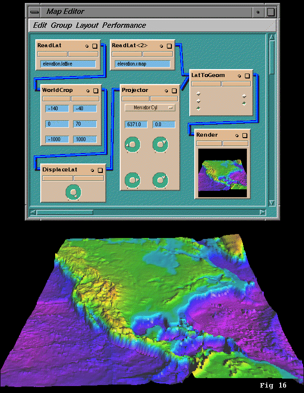
The visualization is shown in Figure 16. A 2-D lattice of elevation data is read in, cropped, and given a third coordinate with the DisplaceLat module. The resulting lattice is then sent through Projector producing a Mercator projection. The LatToGeom module, along with a colormap, then produces the geometry which is displayed by the Render module.

Because of the detail of the data, this visualization ran slowly and consumed in excess of 60 megabytes of memory. Faster updates in the Render window are achived by displaying the image as points when moving the image.

Seismic Tomography

The visualization is shown in Figure 17. The map and bounding box are created and sent to the Projector module. Tomography data is read in as a three-dimensional lattice and sent to the Projector module. This warps the data and map into a sphere and sends the data to two modules which draw isosurfaces. The map and bounding box data is handled as explained above. The isosurfaces are sent to the render module along with geometry output from the SimpleSphere module which simply produces a sphere so that the Earth isn't completely transparent.

This visualization consumed approximately 30 megabytes of memory, most of which was due to the isosurface geometry. Since this particular image required a map of the entire globe, the WorldMap Precision parameter was set to 3600.

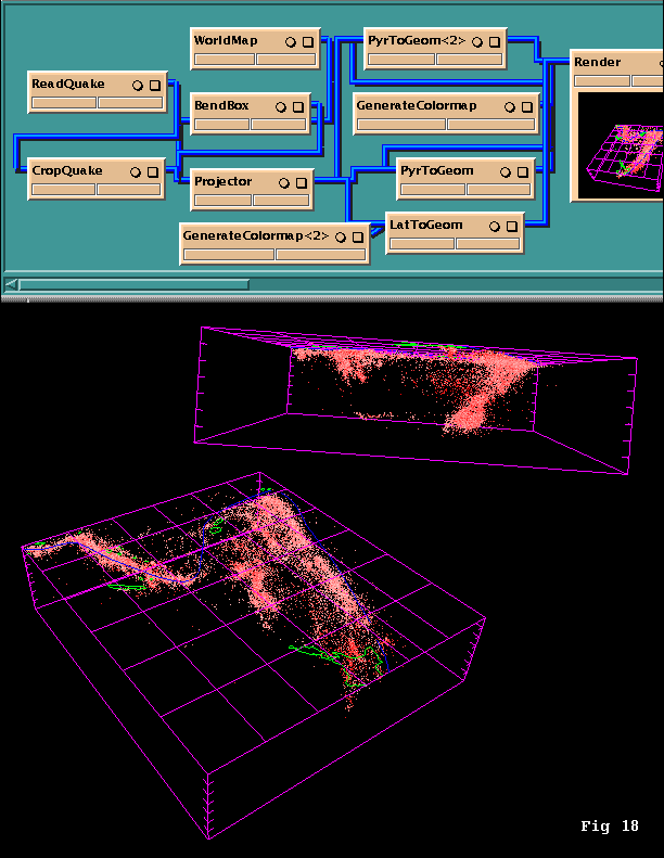
Earthquakes

In this visualization (Figure 18), the earthquakes, map data, and bounding box are read in on the left hand side of the map. Projector takes each of these data types and warps the data onto a Mercator projection. Each data stream is sent to a module which converts the data into colored lines or dots, and then sent to the Render module.

This visualization filled the memory of our 72 megabyte machine, with considerable swapping when all earthquakes were used. This was due to the necessity of storing information for every earthquake in the database and for creating geometry for every earthquake in the cropping region. However, because of the layout of the map and the design of the explorer system, this did not drastically effect the speed of the visualization. Modules such as WorldMap and ReadQuake (the module which read in our quake data) needed to fire only once and could then be swapped out of memory. If necessary to reduce memory demands, these modules could be loaded, fired, connected to other modules so that their output would be passed on, and destroyed.

X. Conclusion

XI. Acknowledgements

The authors wish to thank Drs. Peter van Keken and Dr. Wim Spakman of the University of Utrecht, the Netherlands for providing the earthquake data. The authors also wish to thank Dr. Robert L. Woodward for providing the seismic tomographic data.

XII. References

Morin, P. J., Tanimoto, T., Yuen, D. A., & Zhang, Y. Supercomputing Review vol 5, no 2, Feb 1992, pp. 36-43 and cover. Also appeared as A.H.P.C.R.C. preprint 91-128, 1100 Washington Ave. S, Mpls. MN 55415.

Morin, P. J., Tanimoto, T., Yuen, D. A., & Zhang, Y. Iris Universe 19, pp.50-55 (Winter 1992). Also appeared as A.H.P.C.R.C. preprint 92-023, 1100 Washington Ave. S, Mpls. MN 55415.

Richardus, P. & Adler, R. K. Map Projections For Geodesists, Cartographers and Geographers, North-Holland Publishing Company (1972).

Woodward, R. L., Forte, A. M., Su, W., & Dziewonski, A. M. "Constraints on the Large-Scale Structure of the Earth's Mantle." Preprint, to appear in American Geophysical Union Monograph Series, 1993.

Zhang, Y. & Tanimoto, T. Ridges, hotspots and their interaction as observed is seismic velocity maps, Nature 355, pp. 45-49 (2 Jan. 1992).

Appendix I. Map Feature Color Numbers

 1 Demarcated or delimited international boundary
 2 Indefinite or in dispute international boundary
 3 Other line of separation of sovereignty on land
21 Demarcated or delimited national boundary
22 Indefinite or in dispute national boundary
23 Other national boundary
41 Coasts, islands and lakes that appear on all maps
42 Additional major islands and lakes
43 Intermediate islands and lakes
44 Minor islands and lakes
46 Intermittent major lakes
47 Intermittent minor lakes
48 Reefs
49 Salt pans-major
50 Salt pans-minor
53 Ice shelves-major
54 Ice shelves-minor
55 Glaciers
61 Permanent major rivers
62 Additional major rivers
63 Additional rivers
64 Minor rivers
65 Double lined rivers
66 Intermittent rivers-major
67 Intermittent rivers-additional
68 Intermittent rivers-minor
70 Major canals
71 Canals of lesser importance
72 Canals-irrigation type
81 Plate boundaries
99 Grid lines / BendBox output

Figure Descriptions

Figures 1-6,7-11, 12-14

Examples of various map projections, showing North America and larger regions where appropriate to illustrate properties of the projections.

Figure 15

Explorer map and visualization for a simple map of North America with a bounding box.

Figure 16

Explorer map and visualization for elevation data for North America. Note that the scale is greatly distorted.

Figure 17

Explorer map and visualization for seismic tomography data (Woodward, et. al.). View is of pacific ocean. Isosurfaces represent thermal anomalies of 1000 Kelvin (red) and -1000 Kelvin (blue).

Figure 18

Explorer map and visualization for earthquakes of magnitude three and greater occuring near the Tonga trench.

Figure 19

Map of Minnesota, illustrating level of detail available from WorldMap.

Figure 20

Additional seismic tomography data (Woodward, et. al.), illustrating use of Cassini-Soldner projection for an area of primarily north-south extent. View is of the Americas. Isosurfaces represent thermal anomalies of -2000 Kelvin (light blue), -1500 Kelvin (medium blue), and -1000 Kelvin (dark blue).