Working with Still Frames

In this section, we will look at some of the variety of ways VMD can work with still frames.

Graphical Representation Resolution

Objects are drawn with an adjustable resolution, allowing users to balance fineness of detail with drawing speed. The resolution setting directly controls the smoothness of the surface molecular representation, and the quality of lighting, texturing, and surface shading for interactive display. The resolution setting also affects the quality of external renderers, but with important differences which will be discussed later.

1

Load the files dna.pdb and dna.psf.

2

Show just the DNA, and use the VDW drawing method.

3

Zoom in on one or two of the atoms, either by using the scroll wheel on your mouse, or by using Mouse $\rightarrow$ Scale Mode (shortcut s) and clicking and dragging.

4

Notice that with the default resolution setting, the ``spherical'' atoms aren't looking very spherical. In the Graphical Representations window, click on the representation you set up before for the DNA, and click on the Draw Style tab. Try adjusting the Sphere Resolution setting to something higher, and see what a difference it can make. (See Fig. 2.)

Figure 2: The effect of the resolution setting.

[Low resolution: Sphere Resolution set to 8] [High resolution: Sphere Resolution set to 28]

Many of the drawing methods have a resolution setting. Try a few different ones. When producing images, you can usually raise the resolution until it stops making a visible difference.

Colors and Materials

Nearly all aspects of the display are user-adjustable, including background and display mode colors, and material properties of the objects drawn. Material properties control the way that VMD calculates surface lighting and opacity of displayed objects. Material properties can be used to create dull matte surfaces, eye catching shiny or glass-like surfaces, and transparent ghost-like objects, each suiting different needs. Dull, matte, or diffuse materials are frequently used for background objects or low importance areas of structure, when one wishes to provide context but not draw too much attention, and are also well suited to production of high quality grayscale images. Shiny or glassy materials are useful to attract attention, and emphasize surface curvature with specular highlights. Shiny materials may be too ``busy'' for grayscale images, and tend to be best suited to use in color images. Opacity can be used to deemphasize areas of structure or to provide context, and can be particularly useful when superimposing several objects.

1

In the VMD Main window, choose Graphics $\rightarrow$ Colors.... Look through the Categories list. All display colors, e.g. the color of phosphorus atoms when coloring by name, are set here.

2

Now we will change the background color. In Catagories, select Display. In Names, now click Background. Finally, choose white in Colors.

3

When making a figure for a publication, we often don't want the axes showing. Select Display $\rightarrow$ Axes $\rightarrow$ Off to disable them.

4

You may have noticed the Material menu in the Graphical Representations window. Choose the DNA representation you made above, and experiment with the Material menu.

Figure 3: Examples of different material settings.

[The default transparent material.] 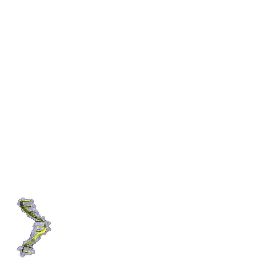[A user-defined material.]

5

Now we'll make a new material. In the VMD Main window, choose Graphics $\rightarrow$ Materials.... In the window that appears, you'll see a list of the materials you just tried out, and their adjustable settings. Click the Create New button, and give it the following settings:

Setting	Value
Ambient	0.62
Diffuse	1.00
Specular	0.87
Shininess	0.85
Opacity	0.11

See if you can reproduce Fig. 3(b) (Hint: use two representations of DNA.)

Depth Perception

Since the systems we are dealing with are three dimensional, VMD has multiple ways of representing the third dimension. In this section we will explore the use of VMD features which enhance or diminish depth perception.

1

The first thing to consider is the projection mode. In the VMD Main window, click the Display menu. Here we can choose either Perspective or Orthographic. In perspective mode, things nearer the camera appear larger. Although perspective projection provides strong size-based visual depth cues, the displayed image will not preserve scale relationships or parallelism of lines, and objects very close to the camera may appear distorted. Orthographic projection preserves scale and parallelism relationships between objects in the displayed image, but greatly reduces depth perception. See Fig. 4 to see the difference this can make.

Figure 4: Comparison of perspective and orthographic projection modes. These were taken from above and to the side of the DNA.

[Perspective] [Orthographic]

2

Another way VMD can represent depth is through so-called ``depth cueing''. Depth cueing is used to enhance three-dimensional perception of molecular structures, particularly with orthographic projections. Choose Display $\rightarrow$ Depth Cueing in the VMD Main window. With depth cueing enabled, objects further from the camera are blended into the background. Depth cue settings are found in Display $\rightarrow$ Display Settings.... Here you can choose the functional dependence of the shading on distance, as well as some parameters for this function.

Figure 5: Stereo image of DNA, also showing linear depth cueing, with Cue Start = 1.5, Cue End = 2.75.

3

Finally, VMD can also produce stereo images. In the VMD Main window, look at the Display $\rightarrow$ Stereo menu, showing many different choices. Choose SideBySide, and return to Perspective mode as well. You should get something like that shown in Fig. 5

Rendering

By now we've seen some techniques for producing attractive figures in VMD interactively. In this section, we'll explore the use of the snapshot feature and external rendering programs to produce high quality image files. The interactive graphics display in VMD is performed by OpenGL and uses fast-but-elementary geometry, lighting, and transparency algorithms. In many cases, the interactive renderings created by VMD are adequate for use in presentations, movies, and small figures. The ``snapshot'' renderer saves the on-screen image and is handy for these cases. When one desires higher quality antialiasing, transparency, lighting, perfectly curved spheres, solid clipped volumes, or extremely high resolution images, renderers such as Tachyon and POV-Ray are better choices. Several of the supported renderers use ray tracing for high quality rendering of curved surfaces. Most of the supported renderers perform lighting calculations at every pixel, and so there's less need to set the graphical representation resolution parameters to high values. Renderers such as Tachyon and POV-Ray actually perform better and create nice images with very conservative representation resolution settings. Other rendering modes such as STL and VRML can be used to export the VMD molecular scene to a variety of rendering and animation tools, or for printing of 3-D solid models.

1

Rendering is a simple matter. Once you have the scene set the way you like it, simply choose File $\rightarrow$ Render... in the VMD Main window. In the File Render Controls window that appears, you choose the renderer to use, choose the file name, and click Start Rendering.

2

Now let's actually render something. Try rendering the scene you have set up currently, using the renderers snapshot, TachyonInternal, and POV3.

3

OK, now for something more challenging. Try to reproduce Fig. 6 as best you can. Think about which parts of the system to show, the drawing and coloring method, the projection mode, and the materials.

Figure 6: Example of POV3 rendering.

Volumetric Data

VMD has the ability to compute and display volumetric data. Volumetric data is data that is a function of position, e.g. density, potential, solvent accessibility, stored as a 3-D grid of values. VMD can display volumetric data in a few different ways. For this section, please turn GLSL rendering off, if it is on.

1

Load the file volmap-density.dx by selecting our molecule in the VMD Main window, clicking File $\rightarrow$ Load Data Into Molecule..., then browsing to the file.

2

Our molecule now has one volumetric data set associated with it, as indicated by the ``1'' in the Vol column of the VMD Main window. Now we need a representation to display it. Create a new representation, and select VolumeSlice as the Drawing Method.

3

With the new representation still selected, set Slice Axis to Y, Render Quality to Medium, and Coloring Method to Volume.

4

Turn off all other representations, then type the following into the Tk Console window:

display resetview
rotate x by -90

Play with the Slice Offset slider, which adjusts the y-coordinate of the slice. Different colors represent different numerical values of the volumetric data, in this case mass density. When coloring by Volume, the color scale can be set in the Trajectory tab of the Graphical Representations window.

Figure 7: Different ways of showing volumetric data of DNA mass density.

[Volume slices.] [Mesh and transparent solid surfaces at isovalue 0.33.]

5

Now make a similar slice representation for the x- and z-directions as well, and rotate you view with the mouse so that all three planes are visible. Fig. 7(a) shows an example with slice planes normal to the x- and y-axes.

6

Now for a more three-dimensional way of representing the data. Hide the current representations, then create a new one using the Isosurface drawing method. In the Draw menu, select Solid Surface. Now, you can see a surface of constant volumetric value, chosen using the Isovalue slider. As you choose higher values, you see the surface shrinks down around a core where the most average mass was located. Fig. 7(b) shows such an isosurface, represented by both a wire mesh and a transparent surface.

7

Another common way to represent volumetric data is by coloring other representations based on it. Load the file pmepot.dx by selecting your current molecule, and choosing File $\rightarrow$ Load Data Into Molecule... in the VMD Main window.

8

Now hide your current representations, and create a new one showing only DNA, with MSMS drawing style and Volume coloring style. The DNA surface is now colored based on the volumetric data value at each surface point. The color scale range is automatically set, but can be changed in the Trajectory tab of the Graphical Representations window.

9

We'll use the Color Scale Bar VMD plugin to show the color scale of the volumetric data. Choose Extensions $\rightarrow$ Visualization $\rightarrow$ Color Scale Bar in the VMD Main window.

10

Enable the Autoscale option, set the label color to black, and click Draw Color Scale Bar. This plugin will create a new molecule named Color Scale Bar that is ``fixed'', meaning when you rotate or scale the scene, the color bar doesn't change.

11

You can move the color bar by unfixing its molecule and fixing the DNA molecule, then using the Translate mouse mode (shortcut T). Recall that a molecule is fixed or unfixed by double-clicking the ``F'' directly to the left of its name in the VMD Main window. An example is shown in Fig. 8.

Figure 8: Example of coloring by volumetric data and use of the Color Scale Bar plugin.

Clipping Planes

In this section, we will learn one of the most useful techniques for producing clear figures: the clipping plane. Clipping planes allow us to look at cross-sections of the objects displayed, and can be applied very flexibly. We will learn how to use them by going through the steps of making Fig. 9.

Figure 9: A three-dimensional contour plot, made through the use of clipping planes.

1

Start a fresh VMD session, and reload the files dna.psf, dna.pdb, and volmap-density.dx.

2

Create the representations in the following table. For each, select Draw $\rightarrow$ Solid Surface and Show $\rightarrow$ Isosurface in the Draw style tab. Once they're set up, you should see only a blue shell.

Drawing Method	Isovalue	Coloring Method
Isosurface	1.0	ColorID 1 (red)
Isosurface	0.6	ColorID 7 (green)
Isosurface	0.2	ColorID 0 (blue)

3

Now enter the following commands in the Tk Console:

mol clipplane status 0 0 0 2
mol clipplane status 0 1 0 2
mol clipplane status 0 2 0 2

Let's decipher this a bit. Every mol clipplane command is of the form

mol clipplane <command> <clipid> <repid> <molid> <value>.

Here, we have used the status command, which we use to enable the clipping planes. Thus, the first line refers to the first clipping plane of the first representation of the first molecule. The final 2 is the new status of each clip plane. Table 1 summarizes this command's usage.

Table 1: Summary of mol clipplane usage.

<command>	Possible <value>s
status	0 (off), 1 (on), 2 (on, solid surface; material inherited from representation)
normal	"<x> <y> <z>", a vector pointing normal to the surface
center	"<x> <y> <z>", a vector pointing to the center of the surface
color	"<r> <g> <b>", an RGB triple specifying the color of the surface, if it is solid

4

Let's check the current settings of the clipping planes. Type the commands:

mol clipplane center 0 0 0
mol clipplane normal 0 0 0

and likewise for the other two clipplanes. By providing no new value, the command now print the current value instead of setting a new one. You should find that all clipplanes are centered at the origin, and with normal vector in the z-direction.

5

Now we'll use a trick to set the center and normal vectors interactively, using the Clipping Plane Tool VMD Plugin. Select Extensions $\rightarrow$ Visualization $\rightarrow$ Clipping Plane Tool in the VMD Main window. This tool will modify clipping planes of the molecules selected in the Apply To menu. The Edit Clip Plane buttons select which clipid will be edited. However, all representation clipping planes will be edited together, i.e. all the clipping planes we've created will get the same normal and center -- exactly what we want.

6

You should now see cross-sections of the isosurfaces you created. Rotate down with the mouse. The clipping plane stays parallel to the screen, letting us choose the normal vector (the flip button inverts this vector). Try to set the normal vector so that we get a nice cross-section of the isosurfaces.

7

Now, adjust the position of the plane in the normal direction by using the Distance slider. Try to cut right through the center of the isosurfaces.

8

When you think you have a nice cross-section, click the Keep Aligned with Screen button to turn this feature off. Now, you can rotate the scene without changing the normal vector, letting you see your work from a different angle.

9

Before we close the Clip Tool window, click the Render plane as solid option near the bottom. This way, the status of our clipping planes will remain 2, as we set in the first step.

10

Now check the center and normal vectors of your clipping planes again, just as you did before. You should find that they have new values. For reference, here are the values used to produce Fig. 9:

Vector	Value
Normal	0.03 0.93 -0.36
Center	0.13 -1.17 13.78

11

Now we'll change the color of the planes to match the rest of the surface, using the following commands:

mol clipplane color 0 0 0 "1 0 0"
mol clipplane color 0 1 0 "0 1 0"
mol clipplane color 0 2 0 "0 0 1"

corresponding to red, green, and blue respectively.

Finally, before rendering, we need to shift two of the planes slightly, so that all three aren't in exactly the same place. Otherwise, we would only see one of the colors.

12

First decide a good shift direction -- just reshow the axes, and see which direction is roughly normal to your planes. For the case of Fig. 9 above, this is the y-direction.

13

Now we'll move the plane for the largest contour 0.1 Å in the direction you chose, and the plane for the smallest contour by 0.1 Å in the opposite direction, using the axes to get the correct sign. You can do this by setting the center to the value you found above, offset by the appropriate amount. For example,

mol clipplane center 0 0 0 "0.13 -1.27 13.78"
mol clipplane center 0 2 0 "0.13 -1.07 13.78"

Now you're ready. Just hide the axes once more, and render using the POV renderer (the other renderers will not show the solid clipping plane surfaces.)

Visualizing Large Systems

Before moving on to trajectory topics, we will very briefly look at a script written by Jordi Cohen that uses volumetric data as a technique for visualizing large systems very clearly.

1

Start a new VMD session, and load the ribosome structure, PDB code 1VS6. Now is a great time to try out VMD's ability to download PDBs directly. If you have an active internet connection, simply type 1VS6 as the Filename in the Molecule File Browser window (menu item File $\rightarrow$ New Molecule...).

2

In the Tk Console, type the following commands:

source marshmallow.tcl
marshmellify

3

This may take a minute or two to complete. When it does, you'll see that many new representations have been created, one for each chain of the ribosome. Examine the script to see how it works -- it is surprisingly short for how much it does.