In this unit you will learn to construct synthetic systems and simulate the passage of ions through a nanopore device.
| cd ``your working directory'' | |
| cd bionano-tutorial-files | |
| cd 1_build | |
| mol new unit_cell_alpha.pdb |
Next, select Graphics ![]() Representations....
In the Graphical Representations window, set the
Drawing Method to CPK. Now we can clearly see the
configuration of atoms in the unit cell. This configuration of eight
nitrogen atoms and six silicon atoms will form the basis for our
extended
Representations....
In the Graphical Representations window, set the
Drawing Method to CPK. Now we can clearly see the
configuration of atoms in the unit cell. This configuration of eight
nitrogen atoms and six silicon atoms will form the basis for our
extended
![]() crystal.
crystal.
|
To generate a crystal membrane from the unit cell, we will
execute a script included with this tutorial. The main steps in the script
are as follows. First, we open an output PDB and write REMARK
lines specifying the geometry of the crystal. Next, we read the unit
cell PDB, extracting the records for each atom. We then generate the
crystal by repeatedly writing the atom records from the unit cell PDB
to the output PDB, albeit with new positions that are displaced by
periodic lattice vectors. In the following part of the tutorial, the
script, replicateCrystal.tcl, we will use to generate the
crystal is presented. Each portion of the script is preceded by text
describing how it works. If you'd like to move on with the tutorial
without examining the details of the script, simply skip ahead to
page ![[*]](crossref.gif) .
.
As will be common to most of the scripts presented in this tutorial,
the first section of the script defines variables that act as the
arguments of the script. The names of input and output files will
often appear here, as in the case below, where the name of the PDB
file containing the crystal's unit cell is stored in unitCellPdb and that of the resultant PDB is stored in outPdb.
The variables n1, n2, and n3 determine the number
of times that the unit cell will be replicated along the respective
crystal axis. The remaining variables describe the geometry of the
unit cell. The unit cell is a parallelepiped with sides of lengths
l1, l2, and l3 along directions given by the unit
vectors basisVector1, basisVector2, and basisVector3. Thus, the set of vectors {![]() ,
,
![]() ,
, ![]() }, where
}, where
![]() , generates the
translational symmetry of the lattice.
, generates the
translational symmetry of the lattice.
replicateCrystal.tcl
# Read the unit cell of a pdb and replicate n1 by n2 by n3 times.
# Input:
set unitCellPdb unit_cell_alpha.pdb
# Output:
set outPdb membrane.pdb
# Parameters:
# Choose n1 and n2 even if you wish to use cutHexagon.tcl.
set n1 6
set n2 6
set n3 6
set l1 7.595
set l2 7.595
set l3 2.902
set basisVector1 [list 1.0 0.0 0.0]
set basisVector2 [list 0.5 [expr sqrt(3.)/2.] 0.0]
set basisVector3 [list 0.0 0.0 1.0]
The two following Tcl procedures extract data from
the PDB. The first returns a list of 3D
vectors corresponding to the {![]()
![]()
![]() } coordinates of each atom
in the unit cell. The second simply extracts each line atom record
from the PDB and returns it as a list.
} coordinates of each atom
in the unit cell. The second simply extracts each line atom record
from the PDB and returns it as a list.
# Return a list with atom positions.
proc extractPdbCoords {pdbFile} {
     set r {}

     # Get the coordinates from the pdb file.
     set in [open $pdbFile r]
     foreach line [split [read $in] \n] {
          if {[string equal [string range $line 0 3] "ATOM"]} {
               set x [string trim [string range $line 30 37]]
               set y [string trim [string range $line 38 45]]
               set z [string trim [string range $line 46 53]]

               lappend r [list $x $y $z]
          }
     }
     close $in
     return $r
}

# Extract all atom records from a pdb file.
proc extractPdbRecords {pdbFile} {
     set in [open $pdbFile r]

     set pdbLine {}
     foreach line [split [read $in] \n] {
          if {[string equal [string range $line 0 3] "ATOM"]} {
               lappend pdbLine $line
          }
     }
     close $in

     return $pdbLine
}
Given the coordinates of all atoms in the unit cell, the displaceCell procedure shifts them by a lattice vector. In other words, this procedure is where the crystal is actually replicated--the basis on which the rest of the script rests.
# Shift a list of vectors by a lattice vector.
proc displaceCell {rUnitName i1 i2 i3 a1 a2 a3} {
     upvar $rUnitName rUnit
     # Compute the new lattice vector.
     set rShift [vecadd [vecscale $i1 $a1] [vecscale $i2 $a2]]
     set rShift [vecadd $rShift [vecscale $i3 $a3]]

     set rRep {}
     foreach r $rUnit {
          lappend rRep [vecadd $r $rShift]
     }
     return $rRep
}
The procedure makePdbLine is essential to the correct formation of the output PDB. The lines of the unit cell PDB obtained by extractPdbRecords are altered to reflect the new coordinates of the translated unit cells.
# Construct a pdb line from a template line, index, resId, and coordinates.
proc makePdbLine {template index resId r} {
     foreach {x y z} $r {break}
     set record "ATOM  "
     set si [string range [format "     %5i " $index] end-5 end]
     set temp0 [string range $template 12 21]
     set resId [string range "    $resId"  end-3 end]
     set temp1 [string range $template  26 29]
     set sx [string range [format "       %8.3f" $x] end-7 end]
     set sy [string range [format "       %8.3f" $y] end-7 end]
     set sz [string range [format "       %8.3f" $z] end-7 end]
     set tempEnd [string range $template 54 end]

     # Construct the pdb line.
     return "${record}${si}${temp0}${resId}${temp1}${sx}${sy}${sz}${tempEnd}"
}
The final procedure drives the script. The series of puts
commands near the top of the procedure store the geometry of the
crystal in REMARK lines in the output PDB. These lines will be
needed later when we modify the shape of the crystal. The lattice
vectors are defined by
# Build the crystal.
proc main {} {
     global unitCellPdb outPdb
     global n1 n2 n3 l1 l2 l3 basisVector1 basisVector2 basisVector3

     set out [open $outPdb w]
     puts $out "REMARK Unit cell dimensions:"
     puts $out "REMARK a1 $a1"
     puts $out "REMARK a2 $a2"
     puts $out "REMARK a3 $a3"
     puts $out "REMARK Basis vectors:"
     puts $out "REMARK basisVector1 $basisVector1"
     puts $out "REMARK basisVector2 $basisVector2"
     puts $out "REMARK basisVector3 $basisVector3"
     puts $out "REMARK replicationCount $n1 $n2 $n3"

     set a1 [vecscale $l1 $basisVector1]
     set a2 [vecscale $l2 $basisVector2]
     set a3 [vecscale $l3 $basisVector3]

     set rUnit [extractPdbCoords $unitCellPdb]
     set pdbLine [extractPdbRecords $unitCellPdb]
     puts "\nReplicating unit $unitCellPdb cell $n1 by $n2 by $n3..."

     # Replicate the unit cell.
     set atom 1
     set resId 1
     for {set k 0} {$k < $n3} {incr k} {
          for {set j 0} {$j < $n2} {incr j} {
               for {set i 0} {$i < $n1} {incr i} {
                    set rRep [displaceCell rUnit $i $j $k $a1 $a2 $a3]

                    # Write each atom.
                    foreach r $rRep l $pdbLine {
                         puts $out [makePdbLine $l $atom $resId $r]
                         incr atom
                    }
                    incr resId

                    if {$resId > 9999} {
                         puts "Warning! Residue overflow."
                         set resId 1
                    }
               }
          }
     }
     puts $out "END"
     close $out

     puts "The file $outPdb was written successfully."
}

main
| mol delete all | |
| mol new membrane.pdb |
| mol delete all | |
| mol new block.pdb |
Our subsequent MD simulations will use periodic boundary conditions,
so the shape of our system must be such that the
![]() lattice matches
at the system's boundaries. A hexagonal prism shape can match this
lattice and is more convenient than the parallelpiped we just created
for housing a nanopore with a roughly circular cross section.
In the script for this
purpose, we first obtain the crystal geometry from the REMARK
lines in the PDB and write a file describing the hexagonal periodic
boundary conditions. Next, for convenience, we shift the crystal so
that its centroid coincides with the origin of the coordinate
system. We finally copy the atom records from the input PDB to the
output PDB, skipping those that do not lie within the hexagonal
prism. If you'd like to skip the details of this script, move on to
page .
lattice matches
at the system's boundaries. A hexagonal prism shape can match this
lattice and is more convenient than the parallelpiped we just created
for housing a nanopore with a roughly circular cross section.
In the script for this
purpose, we first obtain the crystal geometry from the REMARK
lines in the PDB and write a file describing the hexagonal periodic
boundary conditions. Next, for convenience, we shift the crystal so
that its centroid coincides with the origin of the coordinate
system. We finally copy the atom records from the input PDB to the
output PDB, skipping those that do not lie within the hexagonal
prism. If you'd like to skip the details of this script, move on to
page .
The first section again contains what serves as arguments to the script. To save time when the script is altered to act on different files, a file name prefix is defined which gives the output files systematic names based on the name of the input file. In addition to cutting the system to a hexagonal prism, the script cutHexagon.tcl also produces a boundary file (with a .bound extension) that contains the periodic simulation cell vectors needed to form bonds between atoms at the boundaries and run simulations in NAMD.
cutHexagon.tcl
# Remove atoms from a pdb outside of a hexagonal prism
# along the z-axis with a vertex along the x-axis.
# Also write a file with NAMD cellBasisVectors.

set fileNamePrefix membrane
# Input:
set pdbIn ${fileNamePrefix}.pdb
# Output:
set pdbOut ${fileNamePrefix}_hex.pdb
set boundaryFile ${fileNamePrefix}_hex.bound
set pdbTemp tmp.pdb
This procedure executes VMD's measure center method to center the system at the origin, which is done for convenience.
# Write a pdb with the system centered.
proc centerPdb {pdbIn pdbOut} {
     mol new $pdbIn
     set all [atomselect top all]
     set cen [measure center $all]
     $all moveby [vecinvert $cen]
     $all writepdb $pdbOut
     $all delete
     mol delete top
}
The procedure readGeometry extracts the crystal geometry from the REMARK lines we added to the PDB in last script and writes the boundary file mentioned above.
# Read the geometry of the system and write the boundary file.
# Return the radius of the hexagon.
proc readGeometry {pdbFile boundaryFile} {
# Extract the remark lines from the pdb.
mol new $pdbFile
set remarkLines [lindex [molinfo top get remarks] 0]
foreach line [split $remarkLines \n] {
if {![string equal [string range $line 0 5] "REMARK"]} {continue}
set tok [concat [string range $line 7 end]]
set attr [lindex $tok 0]
set val [lrange $tok 1 end]
set remark($attr) $val
puts "$attr = $val"
}
mol delete top
# Deterimine the lattice vectors.
set vector1 [vecscale $remark(basisVector1) $remark(a1)]
set vector2 [vecscale $remark(basisVector2) $remark(a2)]
set vector3 [vecscale $remark(basisVector3) $remark(a3)]
foreach {n1 n2 n3} $remark(replicationCount) {break}
set pbcVector1 [vecadd [vecscale $vector1 [expr $n1/2]] \
[vecscale $vector2 [expr $n2/2]]]
set pbcVector2 [vecadd [vecscale $vector1 [expr -$n1/2] ] \
[vecscale $vector2 [expr $n2]]]
set pbcVector3 [vecscale $vector3 $n3]
puts ""
puts "PERIODIC VECTORS FOR NAMD:"
puts "cellBasisVector1 $pbcVector1"
puts "cellBasisVector2 $pbcVector2"
puts "cellBasisVector3 $pbcVector3"
puts ""
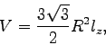
set radius [expr 2.*[lindex $pbcVector1 0]/3.]
puts "The radius of the hexagon: $radius"
# Write the boundary condition file.
set out [open $boundaryFile w]
puts $out "radius $radius"
puts $out "cellBasisVector1 $pbcVector1"
puts $out "cellBasisVector2 $pbcVector2"
puts $out "cellBasisVector3 $pbcVector3"
close $out
return $radius
}
Here, in the procedure cutHexagon, we read each atom record
from the input PDB and extract the serial number and coordinates. The
record is then written to the output PDB if and only if the position
of the atom is within a hexagon of radius ![]() in the
in the ![]() -plane,
centered at the origin, which has a vertex along the
-plane,
centered at the origin, which has a vertex along the ![]() -axis. All
three of the following geometric criteria must hold:
-axis. All
three of the following geometric criteria must hold:
proc cutHexagon {r pdbIn pdbOut} {
     set sqrt3 [expr sqrt(3.0)]

     # Open the pdb to extract the atom records.
     set out [open $pdbOut w]
     set in [open $pdbIn r]
     set atom 1
     foreach line [split [read $in] \n] {
          set string0 [string range $line 0 3]

          # Just write any line that isn't an atom record.
          if {![string match $string0 "ATOM"]} {
               puts $out $line
               continue
          }

          # Extract the relevant pdb fields.
          set serial [string range $line 6 10]
          set x [string range $line 30 37]
          set y [string range $line 38 45]
          set z [string range $line 46 53]

          # Check the hexagon bounds.
          set inHor [expr abs($y) < 0.5*$sqrt3*$r]
          set inPos [expr $y < $sqrt3*($x+$r) && $y > $sqrt3*($x-$r)]
          set inNeg [expr $y < $sqrt3*($r-$x) && $y > $sqrt3*(-$x-$r)]

          # If atom is within the hexagon, write it to the output pdb
          if {$inHor && $inPos && $inNeg} {
               # Make the atom serial number accurate if necessary.
               if {[string is integer [string trim $serial]]} {
                    puts -nonewline $out "ATOM  "
                    puts -nonewline $out \
                    [string range [format "     %5i " $atom] end-5 end]
                    puts $out [string range $line 12 end]

               } else {
                    puts $out $line
               }

               incr atom
          }
     }
     close $in
     close $out
}
In the main part of the script, we extract the radius of the hexagon and write the boundary file, center the crystal, and finally cut the crystal into a hexagonal prism.
set radius [readGeometry $pdbIn $boundaryFile]
centerPdb $pdbIn $pdbTemp
cutHexagon $radius $pdbTemp $pdbOut
| mol delete all | |
| mol load pdb membrane_hex.pdb |
Now we'll shape our crystals into nanopore devices. The script drillPore.tcl has been designed for this purpose. We'll produce a
pore with the shape of two intersecting cones, which has
hourglass-like cross sections in the ![]() - or
- or ![]() - planes. First, we
read the length of the pore along the
- planes. First, we
read the length of the pore along the ![]() -axis from the boundary
file. Subsequently, we remove atoms from the PDB file that are within the
pore. You can skip the details of this script by turning to
page .
-axis from the boundary
file. Subsequently, we remove atoms from the PDB file that are within the
pore. You can skip the details of this script by turning to
page .
The parameters radiusMin and radiusMax define the minimum and maximum radius of the double-cone pore.
drillPore.tcl
# Cut a double-cone pore in a membrane.

# Parameters:
set radiusMin 8
set radiusMax 15
# Input:
set pdbIn membrane_hex.pdb
set boundaryFile membrane_hex.bound
# Output:
set pdbOut pore.pdb
set boundaryOut pore.bound
This procedure extracts the length of the pore along the ![]() -axis,
which is necessary for defining the geometry of the double cone pore.
-axis,
which is necessary for defining the geometry of the double cone pore.
# Get cellBasisVector3_z from the boundary file.
proc readLz {boundaryFile} {
     set in [open $boundaryFile r]
     foreach line [split [read $in] \n] {
          if {[string match "cellBasisVector3 *" $line]} {
               set lz [lindex $line 3]
               break
          }
     }
     close $in
     return $lz
}
In a membrane of thickness ![]() , the cylindrical coordinate
, the cylindrical coordinate ![]() that
corresponds to the radius of the pore at height
that
corresponds to the radius of the pore at height ![]() for a double cone
with a center radius of
for a double cone
with a center radius of
![]() and a maximum radius of
and a maximum radius of
![]() is given by
is given by
# Determine whether the position {x y z} is inside the pore and
# should be deleted.
proc insidePore {x y z sMin sMax} {
     # Get the radius for the double cone at this z-value.
     set s [expr $sMin + 2.0*($sMax-$sMin)/$lz*abs($z)]

     return [expr $x*$x + $y*$y < $s*$s]
}
The final procedure is nearly identical to the cutHexagon procedure in cutHexagon.tcl. It writes only lines satisfying geometrical constraints, this time given by the result of the procedure insidePore.
proc drillPore {sMin sMax lz pdbIn pdbOut} {
     set sqrt3 [expr sqrt(3.0)]

     # Open the pdb to extract the atom records.
     set out [open $pdbOut w]
     set in [open $pdbIn r]
     set atom 1
     foreach line [split [read $in] \n] {
          set string0 [string range $line 0 3]

          # Just write any line that isn't an atom record.
          if {![string match $string0 "ATOM"]} {
               puts $out $line
               continue
          }

          # Extract the relevant pdb fields.
          set serial [string range $line 6 10]
          set x [string range $line 30 37]
          set y [string range $line 38 45]
          set z [string range $line 46 53]

          # If atom is outside the pore, write it to the output pdb.
          # Otherwise, exclude it from the resultant pdb.
          if {![insidePore $x $y $z $sMin $sMax]} {
               # Make the atom serial number accurate if necessary.
               if {[string is integer [string trim $serial]]} {
                    puts -nonewline $out "ATOM  "
                    puts -nonewline $out \
                    [string range [format "     %5i " $atom] end-5 end]
                    puts $out [string range $line 12 end]

               } else {
                    puts $out $line
               }

               incr atom
          }
     }
     close $in
     close $out
}

set lz [readLz $boundaryFile]
drillPore $radiusMin $radiusMax $lz $pdbIn $pdbOut
![\fbox{
\begin{minipage}{.2\textwidth}
\end{minipage} \begin{minipage}[r]{.75\te...
...\textit{Biophysical Journal} \textbf{87}, 2905--2911 (2004)).}
\end{minipage} }](img31.gif)
![\framebox[\textwidth]{
\begin{minipage}[r]{.75\textwidth}
\noindent\small\text...
...udegraphics[width=2.3 cm]{pictures/ypore.png}}
\end{minipage}}
\end{minipage} }](img32.gif)
A quick synopsis of the script's operation is as follows. The first step is to find bonds simply by searching for atoms that are within some threshold distance of one another. However, this step misses bonds that exist across the periodic boundaries. To find these, we displace the system by the periodic cell vectors and find bonds between the original system and its periodic image (Fig. 3). Next we determine the angles and then finally write all of the information to a PSF file.
|
You may be used to calling upon psfgen to produce the structure
files for proteins and other biomolecules. This would be possible for
![]() as well. However, due to the nature of the material, it is
somewhat more straightforward to generate the PSF directly as we do
with this script.
as well. However, due to the nature of the material, it is
somewhat more straightforward to generate the PSF directly as we do
with this script.
![\framebox[\textwidth]{
\begin{minipage}{.2\textwidth}
\end{minipage} \begin{min...
...es
its absolute value, which is negligible for most purposes.}
\end{minipage} }](img33.gif)
To determine the dielectric constant, we will apply an electric field
to a block of
![]() with no free surfaces and measure the electric
dipole moment. Hence, we will use the structure membrane_hex.psf
that we generated in the last section, for which we generated bonds
along all three lattice directions.
with no free surfaces and measure the electric
dipole moment. Hence, we will use the structure membrane_hex.psf
that we generated in the last section, for which we generated bonds
along all three lattice directions.
We take the non-bonded parameters, as well as the values for the
partial charges on the
![]() and
and
![]() atoms in
siliconNitridePsf.tcl, from quantum mechanical calculations
using the biased Hessian method (John A. Wendell and William
A. Goddard III, Journal of Chemical Physics 97,
5048-5062 (1992)). However, the bonded interactions from the same
source lead to a dielectric constant that is practically the same as a
vacuum (1.0). To overcome this, we set the bonded interaction
constants to be much lower than those given in the reference. In this
section, we'll set them to 0.1
atoms in
siliconNitridePsf.tcl, from quantum mechanical calculations
using the biased Hessian method (John A. Wendell and William
A. Goddard III, Journal of Chemical Physics 97,
5048-5062 (1992)). However, the bonded interactions from the same
source lead to a dielectric constant that is practically the same as a
vacuum (1.0). To overcome this, we set the bonded interaction
constants to be much lower than those given in the reference. In this
section, we'll set them to 0.1
![]() . To match
the experimental dielectric constant we include in our force field
harmonic restraints, which can easily be applied in NAMD, that pull
each atom of
. To match
the experimental dielectric constant we include in our force field
harmonic restraints, which can easily be applied in NAMD, that pull
each atom of
![]() towards its equilibrium position in the
towards its equilibrium position in the
![]() crystal. It is the spring constant associated with these constraint
forces that we will calibrate to reproduce the
experimentally-determined dielectric constant of
crystal. It is the spring constant associated with these constraint
forces that we will calibrate to reproduce the
experimentally-determined dielectric constant of
![]() .
.
![\framebox[\textwidth]{
\begin{minipage}{.2\textwidth}
\end{minipage} \begin{min...
...e {\tt chargeSi} in the PSF
generating script (See Appendix).}
\end{minipage} }](img37.gif)
constrainSilicon.tcl
# Add harmonic constraints to silicon nitride.

# Parameters:
# Spring constant in kcal/(mol A^2)
set betaList {1.0}
set selText "resname SIN"
set surfText "(name \"SI.*\" and numbonds<=3) \
or (name \"N.*\" and numbonds<=2)"
# Input:
set psf ../1_build/membrane_hex.psf
set pdb ../1_build/membrane_hex.pdb
# Output:
set restFilePrefix siliconRest

mol load psf $psf pdb $pdb
set selAll [atomselect top all]

# Set the spring constants to zero for all atoms.
$selAll set occupancy 0.0
$selAll set beta 0.0

# Select the silicon nitride.
set selSiN [atomselect top $selText]

# Select the surface.
set selSurf [atomselect top "(${selText}) and (${surfText})"]

foreach beta $betaList {
     # Set the spring constant for SiN to this beta value.
     $selSiN set beta $beta
     # Constrain the surface 10 times more than the bulk.
     $selSurf set beta [expr 10.0*$beta]
     # Write the constraint file.
     $selAll writepdb ${restFilePrefix}_${beta}.pdb
}
$selSiN delete
$selSurf delete
$selAll delete
mol delete top
Before we start, however, we need to put the system dimensions in the NAMD configuration file eq1.namd. Open it and 1_build/membrane_hex.bound (if you did not use InorganicBuilder), which we generated in Section 1.2, in your text editor. If you used InorganicBuilder, refer instead to the vectors you recorded. Copy the values of cellBasisVector1, cellBasisVector2, and cellBasisVector3 into lines 8, 9, and 10, respectively, of the configuration file. Also, examine the constraint parameters at the bottom of the file. Save the configuration file and exit the text editor.
The values of dcdFreq and timestep, taken from the NAMD
configuration file, allow us to determine the time between the frames
of the DCD trajectory file. We'll set the variable startFrame
to 4 to give the system 500 fs to equilbrate before computing the
dipole moment. The electric dipole moment is computed by VMD's measure dipole command which employs the following formula. For a set
of ![]() atoms with partial charges
atoms with partial charges
![]() and positions
and positions ![]() the electric dipole moment is
the electric dipole moment is
dipoleMomentZDiff.tcl
# Calculate dipole moment of the selection
# for a trajectory.

set constraint 10.0
set dcdFreq 100
set selText "all"
set startFrame 0
set timestep 1.0

# Input:
set psf ../1_build/membrane_hex.psf
set dcd field${constraint}.dcd
set dcd0 null${constraint}.dcd
# Output:
set outFile dipole${constraint}.dat

# Get the time change between frames in femtoseconds.
set dt [expr $timestep*$dcdFreq]

# Load the system.
set traj [mol load psf $psf dcd $dcd]
set sel [atomselect $traj $selText]
set traj0 [mol load psf $psf dcd $dcd0]
set sel0 [atomselect $traj0 $selText]

# Choose nFrames to be the smaller of the two.
set nFrames [molinfo $traj get numframes]
set nFrames0 [molinfo $traj0 get numframes]
if {$nFrames0 < $nFrames} {set nFrames $nFrames}
puts [format "Reading %i frames." $nFrames]

# Open the output file.
set out [open $outFile w]

# Start at "startFrame" and move forward, computing
# the dipole moment at each step.
set sum 0.
set sumSq 0.
set n 1
puts "t (ns)\tp_z (e A)\tp0_z (e A)\tp_z-p0_z (e A)"
for {set f $startFrame} {$f < $nFrames && $n > 0} {incr f} {
     $sel frame $f
     $sel0 frame $f

     # Obtain the dipole moment along z.
     set p [measure dipole $sel]
     set p0 [measure dipole $sel0]
     set z [expr [lindex $p 2] - [lindex $p0 2]]

     # Get the time in nanoseconds for this frame.
     set t [expr ($f+0.5)*$dt*1.e-6]

     puts $out "$t $z"
     puts -nonewline [format "FRAME %i: " $f]
     puts "$t\t[lindex $p 2]\t[lindex $p0 2]\t$z"

     set sum [expr $sum + $z]
     set sumSq [expr $sumSq + $z*$z]
}
close $out

# Compute the mean and standard error.
set mean [expr $sum/$nFrames]
set meanSq [expr $sumSq/$nFrames]
set se [expr sqrt(($meanSq - $mean*$mean)/$nFrames)]

puts ""
puts "********Results: "
puts "mean dipole: $mean"
puts "standard error: $se"
mol delete top
mol delete top
This section is only meant to be a demonstration of how the
calibration is performed. Sampling the entire parameter space takes a
good deal of time, but you should now have a good understanding of how
to calibrate the constraints to reproduce the experimental dielectric
constant. In subsequent sections, we will use a parameter file with
the bond constants set to 5.0
![]() and a
constraint file with constants of 1.0
and a
constraint file with constants of 1.0
![]() ,
which have been found to be optimal by the procedure above.
,
which have been found to be optimal by the procedure above.
All biological systems rely on water to function. If our synthetic device is to interact with them, it must be immersed in water.
We'll now remove water from outside of the hexagonal boundaries with the script cutWaterHex.tcl. It uses VMD's atom selection interface to obtain the set {segname, resid, name}, which uniquely specifies each atom, for all atoms violating the geometric constraints that we used in Section 1.2 to cut a hexagon from our crystal. Then by applying the psfgen command delatom, violating atoms are deleted. We estimate the radius of the hexagon with the measure minmax command provided by VMD.
cutWaterHex.tcl
# This script will remove water from psf and pdf outside of a
# hexagonal prism along the z-axis.
package require psfgen 1.3

# Input:
set psf pore_solv.psf
set pdb pore_solv.pdb
# Output:
set psfFinal pore_hex.psf
set pdbFinal pore_hex.pdb

# Parameters:
# The radius of the water hexagon is reduced by "radiusMargin"
# from the pore hexagon. The distance is in angstroms.
set radiusMargin 0.5
# This is the stuff that is removed.
set waterText "water or ions"
# This selection forms the basis for the hexagon.
set selText "resname SIN"

# Load the molecule.
mol load psf $psf pdb $pdb

# Find the system dimensions.
set sel [atomselect top $selText]
set minmax [measure minmax $sel]
$sel delete
set size [vecsub [lindex $minmax 1] [lindex $minmax 0]]
foreach {size_x size_y size_z} $size {break}
# This is the hexagon's radius.
if {[expr $size_x > $size_y]} {
     set rad [expr 0.5*$size_x]
} else {
     set rad [expr 0.5*$size_y]
}
set r [expr $rad - $radiusMargin]

# Find water outside of the hexagon.
set sqrt3 [expr sqrt(3.0)]
# Check the middle rectangle.
set check "($waterText) and ((abs(x) < 0.5*$r and abs(y) > 0.5*$sqrt3*$r) or"
# Check the lines forming the nonhorizontal sides.
set check [concat $check "(y > $sqrt3*(x+$r) or y < $sqrt3*(x-$r) or"]
set check [concat $check "y > $sqrt3*($r-x) or y < $sqrt3*(-x-$r)))"]
set w [atomselect top $check]
set violators [lsort -unique [$w get {segname resid}]]
$w delete

# Remove the offending water molecules.
puts "Deleting the offending water molecules..."
resetpsf
readpsf $psf
coordpdb $pdb
foreach waterMol $violators {
     delatom [lindex $waterMol 0] [lindex $waterMol 1]
}

writepsf $psfFinal
writepdb $pdbFinal
mol delete top
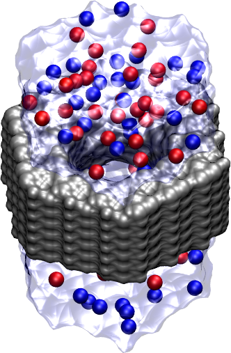
Many biomolecules are sensitive to the ionic strength of the surrounding solvent; therefore, salt is added to the solutions used in experiments to mimic physiological conditions. In addition, ions facilitate measurements of small currents in nanopore systems by substantially increasing the conductivity of the solution.
| mol delete all | |
| mol load psf pore_all.psf pdb pore_all.pdb | |
| set all [atomselect top all] | |
| set minmax [measure minmax $all] | |
| set lz [expr [lindex $minmax 1 2]-[lindex $minmax 0 2]] | |
| $all delete |
The value of lz gives us the size (Å) of the system along the
![]() -axis. We don't want to put this value directly into the NAMD
configuration file, however.
-axis. We don't want to put this value directly into the NAMD
configuration file, however.
It is better for a few water molecules to be crowded at the ends at this point than risk introducing a vacuum region at the ends. While the minimization step can easily rearrange water molecules that have been placed too close together due to wrapping at the periodic boundaries, small regions of vacuum can cause inaccuracies in simulations, especially those performed at constant pressure, that can be difficult to catch.
For this reason, we set cellBasisVector3 to lz minus about 5 Å. Since we get about 55.9 Å for lz, line 13 of eq0.namd should read cellBasisVector3 0.0 0.0 51.0.
| NAMD script | steps | description |
| eq0.namd | 201 | energy minimization |
| eq1.namd | 500 | raise temperature from 0 to 295 K, constant |
| eq2.namd | 1000 | equilibrate, constant |
| run0.namd | 1000 | apply 20 V, constant |
The table above summarizes the NAMD runs we will perform in this section. It consists of three equilibration stages and one run with an applied field. Stages such as these are used in most production simulaions.
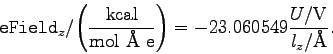
To obtain the value of ![]() , open the NAMD extended system configuration file sample.xsc in your text editor.
Write down c_z, the tenth number in the row of system parameters.
Using
, open the NAMD extended system configuration file sample.xsc in your text editor.
Write down c_z, the tenth number in the row of system parameters.
Using
![]() and
and
![]() , calculate
, calculate
![]() . Note that since the potential difference is applied the along
. Note that since the potential difference is applied the along ![]() -axis,
-axis,
![]() is positive.
is positive.
| eFieldOn on | |
| eField 0.0 0.0 0.0 |
Change the third component of eField to the value of
![]() that you calculated. Before you close the
run0.namd, note that the pressure control lines are absent.
Applying an electric field to a pressure-controlled system will
distort it, leading to erroneous results. In addition, note that the
Langevin temperature control is only applied to the silicon nitride.
Applying Langevin forces to the ions, whose motion due to the electric
field we are trying to measure, could lead to a subtle bias in the
current.
that you calculated. Before you close the
run0.namd, note that the pressure control lines are absent.
Applying an electric field to a pressure-controlled system will
distort it, leading to erroneous results. In addition, note that the
Langevin temperature control is only applied to the silicon nitride.
Applying Langevin forces to the ions, whose motion due to the electric
field we are trying to measure, could lead to a subtle bias in the
current.
|
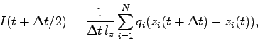
electricCurrentZ.tcl
# Calculate the current for a trajectory.
# Results are in "time(ns) current(nA)"

set dcdFreq 100
set selText "ions"
set startFrame 0
set timestep 1.0

# Input:
set pdb  sample.pdb
set psf  sample.psf
set dcd  run0.dcd
set xsc run0.restart.xsc
# Output:
set outFile curr_20V.dat

# Get the time change between frames in femtoseconds.
set dt [expr $timestep*$dcdFreq]

# Read the system size from the xsc file.
# Note: This only works for lattice vectors along the axes!
set in [open $xsc r]
foreach line [split [read $in] "\n"] {
     if {![string match "#*" $line]} {
          set param [split $line]
          puts $param
          set lx [lindex $param 1]
          set ly [lindex $param 5]
          set lz [lindex $param 9]
          break
     }
}
puts "NOTE: The system size is $lx $ly $lz.\n"
close $in

# Load the system.
mol load psf $psf pdb $pdb
set sel [atomselect top $selText]

# Load the trajectory.
animate delete all
mol addfile $dcd waitfor all
set nFrames [molinfo top get numframes]
puts [format "Reading %i frames." $nFrames]

# Open the output file.
set out [open $outFile w]
#puts $out "sum of q*v for $psf with trajectory $dcd"
#puts $out "t(ns) I(A)"

for {set i 0} {$i < 1} {incr i} {
     # Get the charge of each atom.
     set q [$sel get charge]

     # Get the position data for the first frame.
     molinfo top set frame $startFrame
     set z0 [$sel get z]
}

# Start at "startFrame" and move forward, computing
# current at each step.
set n 1
for {set f [expr $startFrame+1]} {$f < $nFrames && $n > 0} {incr f} {
     molinfo top set frame $f

     # Get the position data for the current frame.
     set z1 [$sel get z]

     # Find the displacements in the z-direction.
     set dz {}
     foreach r0 $z0 r1 $z1 {
          # Compensate for jumps across the periodic cell.
          set z [expr $r1-$r0]
          if {[expr $z > 0.5*$lz]} {set z [expr $z-$lz]}
          if {[expr $z <-0.5*$lz]} {set z [expr $z+$lz]}

          lappend dz $z
     }

     # Compute the average charge*velocity between the two frames.
     set qvsum [expr [vecdot $dz $q] / $dt]

     # We first scale by the system size to obtain the z-current in e/fs.
     set currentZ [expr $qvsum/$lz]
     # Now we convert to nanoamperes.
     set currentZ [expr $currentZ*1.60217733e5]
     # Get the time in nanoseconds for this frame.
     set t [expr ($f+0.5)*$dt*1.e-6]

     # Write the current.
     puts $out "$t $currentZ"
     puts -nonewline [format "FRAME %i: " $f]
     puts "$t $currentZ"

     # Store the postion data for the next computation.
     set z0 $z1
}
close $out
mol delete top
}
![\framebox[\textwidth]{
\begin{minipage}[r]{.75\textwidth}
\noindent\small\text...
...s section. How does
the current compare to double-cone pore? }
\end{minipage} }](img70.gif)
![\fbox{
\begin{minipage}{.2\textwidth}
\end{minipage} \begin{minipage}[r]{.75\te...
... a nanopore can be used to detect
and study single molecules.}
\end{minipage} }](img71.gif)