Next: Non-equilibrium
Up: Analysis
Previous: Analysis
Subsections
This section contains exercises that will let you analyze properties of a system in equilibrium. The exercises mostly use pre-equilibrated trajectories from different ensembles to calculate properties of the ubiquitin system.
RMSD for individual residues
- * 1
- Go to the directory 2-1-rmsd/
You will use a script within VMD that will allow you to compute the average RMSD of each residue in your protein, and assign this value to the User field for each residue.
In the previous unit, you had VMD open with the equilibration trajectory of the ubiquitin periodic system loaded. You will repeat this process:
- * 2
- Load the structure file. First, open the Molecule File Browser from the File
 New Molecule... menu item. Browse for and Load the file ubq_wb.psf in the directory common. (Click ../ to go up one directory.)
- * 3
- The menu at the top of the Molecule File Browser window should
now show 2: ubq_wb.psf. This ensures that the next file that you load will be added to that molecule (molecule ID 2). Now, browse for the file ubq_wb_eq.dcd located in the directory 1-3-box/ and click on Load again. You can close the Molecule File Browser window.
- * 4
- Go to the TkCon window in VMD, and navigate to the 2-1-rmsd/ directory by typing cd ../2-1-rmsd/
- * 5
- The script you will use is called residue_rmsd.tcl. In the TkCon window, type:
This command itself does not actually perform any calculations. It reads the script residue_rmsd.tcl which contains a procedure called rmsd_residue_over_time. Calling this procedure will calculate the average RMSD for each residue you select over all the frames in a trajectory. The procedure is called as:
rmsd_residue_over_time <mol> <sel_resid>
|
|
where <mol> is the molecule in VMD that you select (if not specified, defaults to the top molecule), and <sel_resid> is a list of the residue numbers in that selection. The procedure employs the equations for RMSD shown in Unit 1.
- * 6
- For this example, you will select all the residues in the protein. The
list of residue numbers can be obtained by typing in the TkCon window:
set sel_resid [[atomselect top "protein and alpha"] get resid]
|
|
The above command will get the residue numbers of all the  -carbons in the protein. Since there is just one and only one -carbon per residue, it is a good option. The command will create a list of residue numbers in the variable $sel_resid.
- * 7
- Call the procedure to calculate the RMSD values of all atoms in the newly created selection:
rmsd_residue_over_time top $sel_resid
|
|
You should see the molecule wiggle as each frame gets aligned to the initial structure (This may happen very fast in some machines). At the end of the calculation, you will get a list of the average RMSD per residue. This data is also printed to the file residue_rmsd.dat.
The procedure also sets the value of the User field of all the atoms of the residues in the selection to the computed RMSD value. You will now color the protein according to this value. You will be able to recognize which residues are free to move more and which ones move less during the equilibration.
In order to use these new values to learn about the mobility of the residues, you will create a representation of the protein colored by User value.
- * 8
- Open the Representations window using the Graphics Representations... menu item.
- * 9
- In the Atom Selection window, type protein. Choose Tube as Drawing Method, and in the Coloring Method drop-down menu, choose submenu Trajectory, then User, and again User. Now, click on the Trajectory tab, and in the Color Scale Data Range, type 0.40 and 1.00. Click the Set button.
You should now see the protein colored according to average RMSD values. The residues displayed in blue are more mobile while the ones in red move less. This is somewhat counterintuitive, so you will change the color scale.
- * 10
- Choose the Graphics Colors
 menu item. Choose the Color Scale tab. In the Method pull-down menu, choose BGR. Your figure should now look similar to Fig. 9.
Figure 9:
Ubiquitin colored by the average RMSD per residue. Red denotes more mobile residues, and blue denotes residues which moved less during equilibration.
|
|
- * 11
- Plot the RMSD value per residue by typing in a Terminal window (make sure you are in the directory 2-1-rmsd/):
Take a look at the RMSD distribution. You can see regions where a set of residues shows less mobility. Compare with the structural feature of your protein. You will find a correlation between the location of these regions and secondary structure features like helices or  sheets.
- * 12
- When you are finished investigating the plot, close xmgrace, saving your plot if you wish.
- * 13
- Delete the current displayed molecule in VMD using the VMD Main window by clicking on ubq_wb.psf in the window, and selecting Molecule Delete Molecule.
- * 1
- In a Terminal window, type cd ../2-2-maxwell to change to the directory 2-2-maxwell/
For this exercise, you need a file that contains the velocities of every atom for one instant of the simulation. You will use a file corresponding to the last frame of an equilibration of ubiquitin.
The simulation that generated this file was run exactly as the one you performed in directory 1-3-box/, except that the time step used here was 1fs. You can compare the configuration file used for that simulation to the one in the example-output/ of this directory. As discussed in the first unit, one should use rigidBonds for water in any production simulation since water molecules have been parametrized as rigid molecules. But for the illustration of Maxwell-Boltzmann energy distribution, the effect of force field can be negligible. To be simple, we are not using the option rigidBonds. Here, we provide you with the file ubq_wb_eq_1fs.restart.vel. Alternatively, you can use any velocity file, as long as constraints were not used in the simulation.
- 2
- You will now load the structure file. First, open the Molecule File Browser from the File New Molecule... menu item. Browse for and Load the file ubq_wb.psf in the directory common.
- 3
- The menu at the top of the window should now show 3: ubq_wb.psf. This ensures that the next file that you load will be added to that molecule (molecule ID 3). Now, browse for the file ubq_wb_eq_1fs.restart.vel in the directory 2-2-maxwell/. This time you need to select the type of file. In the Determine file type: pull-down menu, choose NAMD Binary Coordinates, and click on Load again. Close the Molecule File Browser.
The molecule you loaded looks terrible! That is because VMD is reading the velocities as if they were coordinates. It does not matter how it looks, because what we want is to make VMD write a useful file: one that contains the masses and velocities for every atom.
- 4
- In the VMD TkCon window, navigate to the 2-2-maxwell/ directory by typing cd ../2-2-maxwell/
- 5
- First, you will create a selection with all the atoms in the system. Do this by typing in the TkCon window:
set all [atomselect top all]
|
|
- 6
- Now, you will open a file energy.dat for writing:
set fil [open energy.dat w]
|
|
- 7
- For each atom in the system, calculate the kinetic energy
 , and write it to a file
| foreach m [$all get mass] v [$all get {x y z}] { |
|
| puts $fil [expr 0.5 * $m *
[vecdot $v $v] ] |
|
}
|
|
- 8
- Close the file:
- 9
- Outside VMD, take a look at your new energy.dat file. In a Terminal window, make sure you are in the 2-2-maxwell/ directory and type:
It should look something like the list below (although the values will not
necessarily be the same):
| 1.26764386127 |
|
| 0.189726622306 |
|
| 0.268275447408 |
|
...
|
|
- 10
- Quit nedit and VMD.
- * 11
- If you chose not to go through the steps above, there is a VMD script that reproduces them and will create the file energy.dat. In a Terminal Window, type:
vmd -dispdev text -e get_energy.tcl
|
|
This will run VMD in text mode, source the script get_energy.tcl, and produce the energy.dat file. When it is finished, type exit to exit VMD.
You now have a file of raw data that you can use to fit the obtained energy distribution to the Maxwell-Boltzmann distribution. You can obtain the temperature of the distribution from that fit. In the rest of this section, we will show how to do this with the 2-D graphics package xmgrace. If you are more familiar with another tool, you may use it instead.
- * 12
- Quit VMD.
- * 13
- In a Terminal window, type xmgrace.
- * 14
- Once you see the xmgrace window, choose the Data Import ASCII menu item. In the Files box, select the file energy.dat. Click on the OK button. You should see a black trace. This is the raw data. You can now close the Read sets window.
- * 15
- To look at the distribution of points, you will make a histogram of this data. Choose the Data Transformations Histograms... menu item. In the Source Set window, click on the first line, in order to make a histogram of the data you just loaded.
- * 16
- Click on the Normalize option.
- * 17
- Fill in Start: 0, Stop at: 10, and # of bins: 100. Click Apply.
- * 18
- You have created a plot, but you cannot see it yet. Use the right button
of your mouse to click on the first set (in the Source
Set window). Click on Hide. Now, go to the main Grace window and click on the button labeled AS, that will resize
the plot to fit the existing values. This is your distribution of energies.
Figure 10:
Maxwell-Boltzmann distribution for kinetic energies.
![\begin{figure}\begin{center}
\par
\par
\latex{
\includegraphics[scale=0.5]{pictures/tut_unit02_mboltzunix}
}
\end{center}
\end{figure}](img74.png) |
Now, you will fit a Maxwell-Boltzmann distribution to this plot and find out the temperature that the distribution corresponds to. (Hopefully, the temperature you wanted to have in your simulation!)
- * 19
- Choose the Data Transformations Non-linear curve fitting... menu item. In the Source Set window, click on the last line, which corresponds to the histogram you created.
- * 20
- In the Main tab, type in the Formula window:
y = (2/ sqrt(Pi * a0 3 )) * sqrt(x) * exp (-x / a0) 3 )) * sqrt(x) * exp (-x / a0)
|
|
This will fit the curve and get a fit for the parameter a0, which corresponds to  in units of kcal/mol. (These are the energy units that NAMD uses)
- * 21
- In the Parameters drop-down menu, choose 1. Fill-in forms will appear below. You can give an initial value to A0, so that the iterations will look for a value in the vicinity of your initial guess. In the A0 window, type 0.6, which in kcal/mol corresponds to a temperature of
 .
.
- * 22
- Click on the Apply button. This will open a window with the new value for a0, as well as some statistical measures, including the Correlation Coefficient, which is a measure of the fit (better fit as it approaches 1). You can click on the Apply button of the Non-linear fit window several times to obtain a better fit.
- * 23
- The value of a0 you obtained corresponds to . Obtain the temperature
 for this distribution with
 . Your result is hopefully close to
  K!
K!
The deviation from your value and the expected one is due to the poor sampling as well as to the finite size of the protein; the latter implies that temperature can be ``measured'' only with an accuracy of about  even in case of perfect sampling.
- * 24
- When you are finished investigating the histogram and fit, close xmgrace, saving your work if you wish.
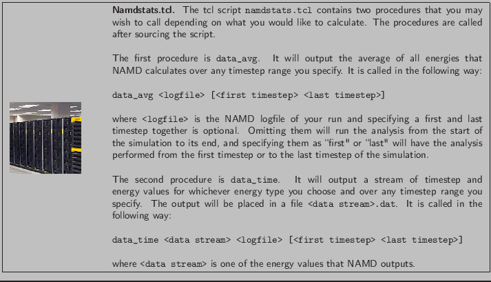
You will look at the kinetic energy and all internal energies: bonded (bonds, angles and dihedrals) and non-bonded (electrostatic, van der Waals) over the course of the water box simulation which you ran in the previous unit. This section will introduce you to a tcl script called namdstats.tcl which is very useful for calculating average energy data for a simulation or extracting energy data over time.
- * 1
- In a Terminal, go to the directory 2-3-energies/
We will investigate the simulation you ran in directory ../1-3-box/. Namdstats.tcl will search all the information in the NAMD output file and extract the energy data for you. You should investigate it with your text editor to familiarize yourself with it.
- * 2
- Open VMD by typing vmd in the Terminal window.
- * 3
- In the VMD TkCon window, navigate to the 2-3-energies/ using the cd command if you are not already there.
- * 4
- To use the script, type
| source namdstats.tcl |
|
data_avg ../1-3-box/ubq_wb_eq.log 101 last
|
|
The first line will source the script itself, and the second will call a procedure which will calculate the average for all output variables in the log file from the first logged timestep after 101 to the end of the simulation.
- * 5
- The output of namdstats.tcl should appear similar to that in Table 1. Note that the standard units used by NAMD are Å for length, kcal/mol for energy, Kelvin for temperature, and bar for pressure.
| BOND: |
232.561128 |
| ANGLE: |
690.805988 |
| DIHED: |
397.649676 |
| IMPRP: |
41.250136 |
| ELECT: |
-23674.863868 |
| VDW: |
1541.108344 |
| BOUNDARY: |
0.0 |
| MISC: |
0.0 |
| KINETIC: |
4579.147764 |
| TOTAL: |
-16192.340832 |
| TEMP: |
313.429264 |
| TOTAL2: |
-16173.821268 |
| TOTAL3: |
-16174.663916 |
| TEMPAVG: |
313.140436 |
| PRESSURE: |
-47.513352 |
| GPRESSURE: |
-19.105588 |
| VOLUME: |
71087.006196 |
| PRESSAVG: |
3.340104 |
| GPRESSAVG: |
3.4207 |

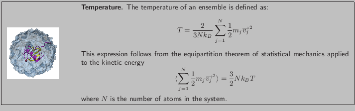
The temperature of your system should be close to 310 K, the temperature we specified for the water box simulation. It will not be exact because temperature fluctuations occur due to the finite size of the system. We will investigate these fluctuations in the next section.
- * 1
- In a Terminal window, go to the directory 2-4-temp/.
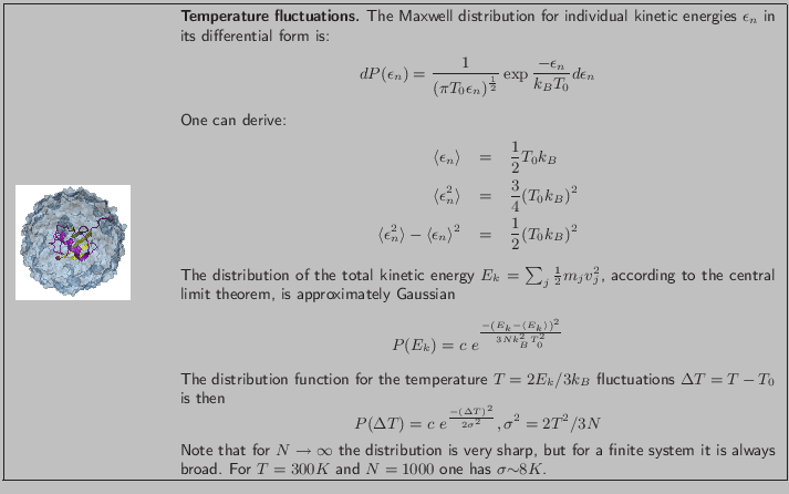
For this exercise, you need a simulation that is long enough to sample the quantity of interest very well. Here, we need to sample the fluctuations in kinetic energy, and hence in the temperature. Instead of doing such a simulation yourself, we recommend that you use the provided file example-output/ubq-nve.log. However, if you choose to run your own simulation, you can find all the necessary files and instructions below. We recommend that you read the whole section even if you don't perform the simulations.
The simulation is performed in the microcanonical ensemble (NVE, i.e., constant number, volume, and energy). The configuration file provided to start the NAMD run is called ubq-nve.conf. The main features of this configuration file are:
- The simulation takes the restart files from the sphere equilibration simulation performed in Unit 1. The files are located in directory 1-2-sphere/ and are named ubq_ws, i.e., ubq_ws.restart.vel, etc.
- The initial temperature is determined by the velocity restart file as shown in equation above. This initial temperature corresponds to
 K, the temperature of the water sphere simulation.
- The time step is 2 fs; with rigidBonds turned on, this time step is acceptable.
- The simulation will run for 1 ns.
- 2
- Run the Molecular Dynamics simulation
- * 3
- If you do not run the simulation yourself, you will need to obtain the data for the temperature from the provided log file. Copy this log file from the directory example-output/.
cp example-output/ubq-nve.log .
|
|
If you run the simulation yourself, your log file will be generated by NAMD, and you do not need to copy it.
- * 4
- In the VMD TkCon window, navigate to the 2-4-temp/ directory by typing cd ../2-4-temp/
- * 5
- In order to obtain the data for the temperature from the log file we will again use the script namdstats.tcl, which we have already sourced. Do this by typing:
data_time TEMP ubq-nve.log
|
|
Each timestep and the corresponding temperature of the system is now in the file TEMP.dat. The script will include all timesteps and it may take some time to finish. Note there is no minimization of the system since this was already performed in the initial simulation.
In order to plot the data, you can use xmgrace.
- * 6
- Open xmgrace.
- * 7
- Choose the Data Import ASCII menu item. Select the file TEMP.dat You should see a black trace. This is a plot of the temperature over time.
- * 8
- To look at the distribution of points, you will make a histogram with this data. Choose the Data Transformations Histograms... menu item. In the Source Set window, click on the first line, in order to make a histogram of the data you just loaded.
- * 9
- Click on the Normalize option, and fill in Start: 300, Stop at: 330, and # of bins 100. Click Apply.
- * 10
- You created a plot, but you cannot see it yet. Use the right button of your mouse to click on the first set (in the Source Set window). Click on Hide. Now, go to the Main window and click on the button labeled AS, that will resize the plot to fit the existing values. This is your distribution of temperatures.
Does this distribution look any familiar? Your distribution should look like a Gaussian distribution.
- * 11
- You will now fit your distribution to a normal distribution. For this, you will use the Non-linear curve fitting feature of xmgrace.
- * 12
- Choose the Data Transformations Non-linear curve fitting... menu item. In the Source Set window, click on the last line, which corresponds to the histogram you created.
- * 13
- In the Main tab, type in the Formula window:
y= a0 * exp(-(x-a1)2/a2)
- * 14
- In the Parameters drop-down menu, choose 3. Fill-in frames will appear below. Give A0 an initial value of 1, A1 an initial value of 315 (you can see that the center of the Gaussian is around that value), and A2 a value of 2. Click several times on the Apply, to get a better fit.
This will fit the curve and get values for the parameters a0, a1 and a2, where a0 is a normalization constant, a1 the average temperature, and a2 is  .
.
Figure 11:
Fluctuation of Temperature in a Finite Sample
![\begin{figure}\begin{center}
\par
\par
\latex{
\includegraphics[scale=0.5]{pictures/tut_unit02_tempunix}
}
\end{center}
\end{figure}](img94.png) |
The window that appeared contains the new value of the parameters, as well as some statistical measures, including the Correlation Coefficient, which is a measure of the fit.
- * 15
- Compare the average value of the temperature obtained by this method with the one you would obtain using namdstats by typing in the VMD TkCon window:
- * 16
- Now, look at the deviation
 which can be calculated from your data. Note how it is dependent on the size of the system!
Take home message: You may note from this example that single proteins, on one hand, behave like infinite thermodynamic ensembles, reproducing the respective mean temperature. On the other hand, they show signs of their finiteness in the form of temperature fluctuations. In general, it is interesting to note that the velocities of the atoms and, therefore, the kinetic energy of the protein serves as its thermometer!
- * 17
- When you are finished investigating the histogram and fit, close xmgrace, saving your work if you wish.
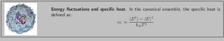
Specific heat is an important property of thermodynamic systems. It is the amount of heat needed to raise the temperature of an object per degree of temperature increase per unit mass, and a sensitive measure of the degree of order in a system. (Near a bistable point, the specific heat becomes large.)
For this exercise, you need to carry out a long simulation in the NVT (canonical) ensemble that samples sufficiently the averages
 and
and
 that arise in the definition of
  . To produce the data for the total energy of the molecule over time, you need to work through the steps presented below. This exercise is long and computationally intensive. You may wish to work only through the steps marked with *, that correspond to the analysis of the data. Nevertheless, we encourage you to read through the whole section since it will provide you with tools for future analysis.
- * 1
- In a Terminal windows, change to the directory 2-5-spec-heat/.
In order to produce an NVT run, you will restart the equilibration you performed in Unit 1 for the water sphere. All necessary files are present in your directory.
- 2
- Run the Molecular Dynamics simulation
- * 3
- If you do not run the simulation yourself, you will need to obtain the trajectory that has been provided. Copy the simulation output from the directory example-output/ by typing in a Terminal window:
cp example-output/ubq-nvt* .
|
|
If you run the simulation yourself, your output will be generated by NAMD, and you do not need to copy it.
You now have an equilibration run of ubiquitin in the NVT ensemble, and you want to look at the fluctuation in the energy of ubiquitin. In order to calculate the specific heat for the protein only (as opposed to the whole system), you need the total energies for the atoms in the protein only, however the NAMD output for the run you just performed contains the energies for all atoms in the system.
You would like NAMD to write the energies for only a part of the system, rather than for the entire system, as is reported in the log file. One way to do this is to run a separate simulation with only the part of the system you are interested in, but this may be unrealistic from a biological standpoint. Fortunately, VMD has a plugin which will call NAMD and allow you to calculate energies for any part of your system that you specify.
- * 4
- In the VMD TkCon window, navigate to the 2-5-spec-heat/ directory:
- * 5
- If you did not run the simulation, and copied output from the example-output directory, please skip this step. If you ran the simulation yourself, perform this step and skip the next one.
Load the psf file and trajectory for your system.
| mol new ../common/ubq_ws.psf |
|
mol addfile ubq-nvt.dcd
|
|
- * 6
- Load the psf file and trajectory for the example-output system.
| mol new ../common/example-output/ubq_ws.psf |
|
mol addfile ubq-nvt.dcd
|
|
- * 7
- In the VMD Main window, open the NAMD Energy plugin by clicking Extensions Analysis NAMD Energy.
Figure 12:
NAMD Energy GUI (Graphical User Interface)
![\begin{figure}\begin{center}
\par
\par
\latex{
\includegraphics[scale=0.5]{pictures/tut_unit02_namdenergy}
}
\end{center}
\end{figure}](img103.png) |
- * 8
- In the NAMDEnergy window, select the following inputs:
- Molecule: ubq_ws.psf
- Selection 1: protein
- Energy Type: ALL
- Output File: myenergy.dat
- Parameter Files: ../common/par_all27_prot_lipid.inp
All other parameters are chosen by default and are consistent with the specifications of your simulation. For more information on NAMD Energy's options, click Help Help...
- * 9
- Click Run NAMDEnergy to perform the analysis. Output will be written in the vmd console window. When you are finished, close the NAMDEnergy window. (Note that NAMD Energy may give you an error message if it cannot find NAMD installed. You may need to point it to the location of NAMD on your computer.) This analysis may take several minutes to be completed.
Now you have a file called myenergy.dat which contains the energy of only the ubiquitin protein atoms in your system. In order to calculate the specific heat of the molecule, we must derive both the average and squared-average total energy of the molecule from this data. We will use a tcl script to do so.
- * 10
- In the VMD TkCon window, source the script to calculate the average total energy of ubiquitin for your simulation:
The script will search your output file for the total energy data for the system, calculate both the average and squared-average total energy over all timesteps, and output the values for you. You should become familiar with the script to fully utilize the power of Tcl scripting in analyzing NAMD output. This script will teach you how to read input files, extract data from them, and perform calculations on that data.
- * 11
- Calculate the specific heat for ubiquitin using the equation provided in
the Energy fluctuations and specific heat box at the beginning of
this section. Consider
and
 K. What is your result? Try to convert your results to units of specific heat used everyday, i.e.,
 using the conversion factor
 . Note that this units correspond to the specific heat per unit mass. You calculated the fluctuation in the energy of the whole protein, so you must take into account the mass of your protein by dividing your obtained value by
 . Compare with some specific heats that are given to you in Table 2.
| Substance |
Specific Heat |
| |
|
| Human Body(average) |
3470 |
| Wood |
1700 |
| Water |
4180 |
| Alcohol |
2400 |
| Ice |
2100 |
| Gold |
130 |
| Strawberries |
3890 |

- * 12
- Delete the current displayed molecule in VMD using the VMD Main window by clicking on ubq_ws.psf in the window, and selecting Molecule Delete Molecule.
Next: Non-equilibrium
Up: Analysis
Previous: Analysis
namd@ks.uiuc.edu
![\framebox[\textwidth]{
\begin{minipage}{.2\textwidth}
\includegraphics[width=2...
... contain pertinent PDB information!) like the User field can.}
\end{minipage} }](img71.png)
![\framebox[\textwidth]{
\begin{minipage}{.2\textwidth}
\includegraphics[width=2...
...utilities/}{http://www.ks.uiuc.edu/Research/namd/utilities/}}}
\end{minipage} }](img84.png)