


Next: Metadynamics
Up: Biasing and analysis methods
Previous: Adaptive Biasing Force
Contents
Index
Subsections
Extended-system Adaptive Biasing Force (eABF)
Extended-system ABF (eABF) is a variant of ABF (13.5.1)
where the bias is not applied
directly to the collective variable, but to an extended coordinate (``fictitious variable'')
 that evolves dynamically according to Newtonian or Langevin dynamics.
Such an extended coordinate is enabled for a given colvar using the
extendedLagrangian and associated keywords (13.2.4).
The theory of eABF and the present implementation are documented in detail
in reference [58].
that evolves dynamically according to Newtonian or Langevin dynamics.
Such an extended coordinate is enabled for a given colvar using the
extendedLagrangian and associated keywords (13.2.4).
The theory of eABF and the present implementation are documented in detail
in reference [58].
Defining an ABF bias on a colvar wherein the extendedLagrangian option
is active will perform eABF; there is no dedicated option.
The extended variable
is coupled to the colvar  by the harmonic potential
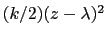 .
Under eABF dynamics, the adaptive bias on
is
the running estimate of the average spring force:
.
Under eABF dynamics, the adaptive bias on
is
the running estimate of the average spring force:
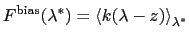 |
(13.20) |
where the angle brackets indicate a canonical average conditioned by
 .
At long simulation times, eABF produces a flat histogram of the extended variable
,
and a flattened histogram of
.
At long simulation times, eABF produces a flat histogram of the extended variable
,
and a flattened histogram of  , whose exact shape depends on the strength of the coupling
as defined by extendedFluctuation in the colvar.
Coupling should be somewhat loose for faster exploration and convergence, but strong
enough that the bias does help overcome barriers along the colvar
.[58]
Distribution of the colvar may be assessed by plotting its histogram, which
is written to the outputName.zcount file in every eABF simulation.
Note that a histogram bias (13.5.7)
applied to an extended-Lagrangian colvar
will access the extended degree of freedom
, not the original colvar
;
however, the joint histogram may be explicitly requested by listing the name of the
colvar twice in a row within the colvars parameter of the histogram block.
, whose exact shape depends on the strength of the coupling
as defined by extendedFluctuation in the colvar.
Coupling should be somewhat loose for faster exploration and convergence, but strong
enough that the bias does help overcome barriers along the colvar
.[58]
Distribution of the colvar may be assessed by plotting its histogram, which
is written to the outputName.zcount file in every eABF simulation.
Note that a histogram bias (13.5.7)
applied to an extended-Lagrangian colvar
will access the extended degree of freedom
, not the original colvar
;
however, the joint histogram may be explicitly requested by listing the name of the
colvar twice in a row within the colvars parameter of the histogram block.
The eABF PMF is that of the coordinate
, it is not exactly the free energy profile of
.
That quantity can be calculated based on the CZAR
estimator.
The corrected z-averaged restraint (CZAR) estimator
is described in detail in reference [58].
It is computed automatically in eABF simulations,
regardless of the number of colvars involved.
Note that ABF may also be applied on a combination of extended and non-extended
colvars; in that case, CZAR still provides an unbiased estimate of the free energy gradient.
CZAR estimates the free energy gradient as:
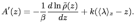 |
(13.21) |
where
is the colvar,
is the extended variable harmonically
coupled to  with a force constant
  , and
, and
 is the observed
distribution (histogram) of
, affected by the eABF bias.
is the observed
distribution (histogram) of
, affected by the eABF bias.
There is only one optional parameter to the CZAR estimator:
-
writeCZARwindowFile
 Write internal data from CZAR to a separate file?
Context: abf
Acceptable values: boolean
Default value: no
Description: When this option is enabled, eABF simulations will write a file containing the
-averaged restraint force under the name outputName.zgrad.
The same information is always included in the colvars state file, which is sufficient
for restarting an eABF simulation.
These separate file is only useful when joining adjacent windows from a stratified
eABF simulation, either to continue the simulation in a broader window or to
compute a CZAR estimate of the PMF over the full range of the coordinate(s).
Similar to ABF, the CZAR estimator produces two output files in multicolumn text format:
- outputName.czar.grad: current estimate of the free energy gradient (grid),
in multicolumn;
- outputName.czar.pmf: only for one-dimensional calculations, integrated
free energy profile or PMF.
The sampling histogram associated with the CZAR estimator is the
-histogram,
which is written in the file outputName.zcount.
Next: Metadynamics
Up: Biasing and analysis methods
Previous: Adaptive Biasing Force
Contents
Index
vmd@ks.uiuc.edu