


Next: Syntax changes from older
Up: Collective Variable-based Calculations (Colvars)
Previous: Selecting atoms
Contents
Index
Subsections
Biasing and analysis methods
All of the biasing and analysis methods implemented recognize the following options:
In addition, restraint biases (9.5.4, 9.5.6, 9.5.7, ...) and metadynamics biases (9.5.3) offer the following optional keywords, which allow the use of thermodynamic integration (TI) to compute potentials of mean force (PMFs). In adaptive biasing force (ABF) biases (9.5.1) the same keywords are not recognized because their functionality is always included.
Adaptive Biasing Force
For a full description of the Adaptive Biasing Force method, see
reference [27]. For details about this implementation,
see references [42] and [43]. When
publishing research that makes use of this functionality, please cite
references [27] and [43].
An alternate usage of this feature is the application of custom
tabulated biasing potentials to one or more colvars. See
inputPrefix and updateBias below.
Combining ABF with the extended Lagrangian feature (9.3.10)
of the variables produces the extended-system ABF variant of the method
(9.5.2).
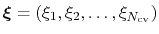
ABF is based on the thermodynamic integration (TI) scheme for
computing free energy profiles. The free energy as a function
of a set of collective variables
![$ {\mbox{\boldmath {$\xi$}}}=(\xi_{i})_{i\in[1,n]}$](img394.png) is defined from the canonical distribution of
is defined from the canonical distribution of
 ,
,
 :
:
 |
(48) |
In the TI formalism, the free energy is obtained from its gradient,
which is generally calculated in the form of the average of a force
 exerted on
, taken over an iso-
surface:
exerted on
, taken over an iso-
surface:
 |
(49) |
Several formulae that take the form of (50) have been
proposed. This implementation relies partly on the classic
formulation [18], and partly on a more versatile scheme
originating in a work by Ruiz-Montero et al. [84],
generalized by den Otter [28] and extended to multiple
variables by Ciccotti et al. [23]. Consider a system
subject to constraints of the form
 . Let
(
. Let
(
![$ {\mbox{\boldmath {$v$}}}_{i})_{i\in[1,n]}$](img401.png) be arbitrarily chosen vector fields
(
be arbitrarily chosen vector fields
(
 ) verifying, for all
  ,
,
 , and
, and  :
:
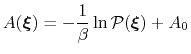
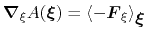
then the following holds [23]:
 |
(52) |
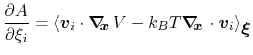
where  is the potential energy function.
 can be interpreted as the direction along which the force
acting on variable
can be interpreted as the direction along which the force
acting on variable  is measured, whereas the second term in the
average corresponds to the geometric entropy contribution that appears
as a Jacobian correction in the classic formalism [18].
Condition (51) states that the direction along
which the total force on
is measured is orthogonal to the
gradient of
is measured, whereas the second term in the
average corresponds to the geometric entropy contribution that appears
as a Jacobian correction in the classic formalism [18].
Condition (51) states that the direction along
which the total force on
is measured is orthogonal to the
gradient of  , which means that the force measured on
does not act on
.
, which means that the force measured on
does not act on
.
Equation (52) implies that constraint forces
are orthogonal to the directions along which the free energy gradient is
measured, so that the measurement is effectively performed on unconstrained
degrees of freedom.
In NAMD, constraints are typically applied to the lengths of
bonds involving hydrogen atoms, for example in TIP3P water molecules (parameter rigidBonds, section 5.6.1).
In the framework of ABF,
 is accumulated in bins of finite size
 ,
thereby providing an estimate of the free energy gradient
according to equation (50).
The biasing force applied along the collective variables
to overcome free energy barriers is calculated as:
,
thereby providing an estimate of the free energy gradient
according to equation (50).
The biasing force applied along the collective variables
to overcome free energy barriers is calculated as:
where

 denotes the current estimate of the
free energy gradient at the current point
in the collective
variable subspace, and
denotes the current estimate of the
free energy gradient at the current point
in the collective
variable subspace, and
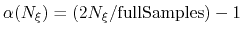
 is a scaling factor that is ramped
from 0 to 1 as the local number of samples
is a scaling factor that is ramped
from 0 to 1 as the local number of samples  increases
to prevent nonequilibrium effects in the early phase of the simulation,
when the gradient estimate has a large variance.
See the fullSamples parameter below for details.
increases
to prevent nonequilibrium effects in the early phase of the simulation,
when the gradient estimate has a large variance.
See the fullSamples parameter below for details.
As sampling of the phase space proceeds, the estimate
is progressively refined. The biasing
force introduced in the equations of motion guarantees that in
the bin centered around
,
the forces acting along the selected collective variables average
to zero over time. Eventually, as the undelying free energy surface is canceled
by the adaptive bias, evolution of the system along
is governed mainly by diffusion.
Although this implementation of ABF can in principle be used in
arbitrary dimension, a higher-dimension collective variable space is likely
to result in sampling difficulties.
Most commonly, the number of variables is one or two.
ABF requirements on collective variables
The following conditions must be met for an ABF simulation to be possible and
to produce an accurate estimate of the free energy profile.
Note that these requirements do not apply when using the extended-system
ABF method (9.5.2).
- Only linear combinations of colvar components can be used in ABF calculations.
- Availability of total forces is necessary. The following colvar components
can be used in ABF calculations:
distance, distance_xy, distance_z, angle,
dihedral, gyration, rmsd and eigenvector.
Atom groups may not be replaced by dummy atoms, unless they are excluded
from the force measurement by specifying oneSiteTotalForce, if available.
- Mutual orthogonality of colvars. In a multidimensional ABF calculation,
equation (51) must be satisfied for any two colvars
and
.
Various cases fulfill this orthogonality condition:
-
and
are based on non-overlapping sets of atoms.
- atoms involved in the force measurement on
do not participate in
the definition of
. This can be obtained using the option oneSiteTotalForce
of the distance, angle, and dihedral components
(example: Ramachandran angles
 ,
,  ).
).
-
and
are orthogonal by construction. Useful cases are the sum and
difference of two components, or distance_z and distance_xy using the same axis.
- Mutual orthogonality of components: when several components are combined into a colvar,
it is assumed that their vectors
(equation (53))
are mutually orthogonal. The cases described for colvars in the previous paragraph apply.
- Orthogonality of colvars and constraints: equation 52 can
be satisfied in two simple ways, if either no constrained atoms are involved in the force measurement
(see point 3 above) or pairs of atoms joined by a constrained bond are part of an atom group
which only intervenes through its center (center of mass or geometric center) in the force measurement.
In the latter case, the contributions of the two atoms to the left-hand side of equation 52
cancel out. For example, all atoms of a rigid TIP3P water molecule can safely be included in an atom
group used in a distance component.
Parameters for ABF
ABF depends on parameters from collective variables to define the grid on which free
energy gradients are computed. In the direction of each colvar, the grid ranges from
lowerBoundary to upperBoundary, and the bin width (grid spacing)
is set by the width (see 9.3.8) parameter.
The following specific parameters can be set in the ABF configuration block:
-
name: see definition of name in sec. 9.5 (biasing and analysis methods)
-
colvars: see definition of colvars in sec. 9.5 (biasing and analysis methods)
- fullSamples
 Number of samples in a bin prior
to application of the ABF
Number of samples in a bin prior
to application of the ABF 
Context: abf
Acceptable Values: positive integer
Default Value: 200
Description: To avoid nonequilibrium effects due to large fluctuations of the force exerted along the
colvars, it is recommended to apply a biasing force only after a the estimate has started
converging. If fullSamples is non-zero, the applied biasing force is scaled by a factor
between 0 and 1.
If the number of samples
in the current bin is higher than fullSamples,
the factor is one. If it is less than half of fullSamples, the factor is zero and
no bias is applied. Between those two thresholds, the factor follows a linear ramp from
0 to 1:
 .
.
- maxForce
Maximum magnitude of the ABF force
Context: abf
Acceptable Values: positive decimals (one per colvar)
Default Value: disabled
Description: This option enforces a cap on the magnitude of the biasing force effectively applied
by this ABF bias on each colvar. This can be useful in the presence of singularities
in the PMF such as hard walls, where the discretization of the average force becomes
very inaccurate, causing the colvar's diffusion to get ``stuck'' at the singularity.
To enable this cap, provide one non-negative value for each colvar. The unit of force
is kcal/mol divided by the colvar unit.
- hideJacobian
Remove geometric entropy term from calculated
free energy gradient?
Context: abf
Acceptable Values: boolean
Default Value: no
Description: In a few special cases, most notably distance-based variables, an alternate definition of
the potential of mean force is traditionally used, which excludes the Jacobian
term describing the effect of geometric entropy on the distribution of the variable.
This results, for example, in particle-particle potentials of mean force being flat
at large separations.
Setting this parameter to yes causes the output data to follow that convention,
by removing this contribution from the output gradients while
applying internally the corresponding correction to ensure uniform sampling.
It is not allowed for colvars with multiple components.
- outputFreq
Frequency (in timesteps) at which ABF data files are refreshed
Context: abf
Acceptable Values: positive integer
Default Value: Colvars module restart frequency
Description: The files containing the free energy gradient estimate and sampling histogram
(and the PMF in one-dimensional calculations) are written on disk at the given
time interval.
- historyFreq
Frequency (in timesteps) at which ABF history files are
accumulated
Context: abf
Acceptable Values: positive integer
Default Value: 0
Description: If this number is non-zero, the free energy gradient estimate and sampling histogram
(and the PMF in one-dimensional calculations) are appended to files on disk at
the given time interval. History file names use the same prefix as output files, with
``.hist'' appended.
- inputPrefix
Filename prefix for reading ABF data
Context: abf
Acceptable Values: list of strings
Description: If this parameter is set, for each item in the list, ABF tries to read
a gradient and a sampling files named
inputPrefix
.grad
and
inputPrefix
.count. This is done at
startup and sets the initial state of the ABF algorithm.
The data from all provided files is combined appropriately.
Also, the grid definition (min and max values, width) need not be the same
that for the current run. This command is useful to piece together
data from simulations in different regions of collective variable space,
or change the colvar boundary values and widths. Note that it is not
recommended to use it to switch to a smaller width, as that will leave
some bins empty in the finer data grid.
This option is NOT compatible with reading the data from a restart file (colvarsInput option of the NAMD config file).
- applyBias
Apply the ABF bias?
Context: abf
Acceptable Values: boolean
Default Value: yes
Description: If this is set to no, the calculation proceeds normally but the adaptive
biasing force is not applied. Data is still collected to compute
the free energy gradient. This is mostly intended for testing purposes, and should
not be used in routine simulations.
- updateBias
Update the ABF bias?
Context: abf
Acceptable Values: boolean
Default Value: yes
Description: If this is set to no, the initial biasing force (e.g. read from a restart file or
through inputPrefix) is not updated during the simulation.
As a result, a constant bias is applied. This can be used to apply a custom, tabulated
biasing potential to any combination of colvars. To that effect, one should prepare
a gradient file containing the gradient of the potential to be applied (negative
of the bias force), and a count file containing only values greater than
fullSamples. These files must match the grid parameters of the colvars.
Multiple-replica ABF
Output files
The ABF bias produces the following files, all in multicolumn text format:
- outputName.grad: current estimate of the free energy gradient (grid),
in multicolumn;
- outputName.count: histogram of samples collected, on the same grid;
- outputName.pmf: only for one-dimensional calculations, integrated
free energy profile or PMF.
If several ABF biases are defined concurrently, their name is inserted to produce
unique filenames for output, as in outputName.abf1.grad.
This should not be done routinely and could lead to meaningless results:
only do it if you know what you are doing!
If the colvar space has been partitioned into sections (windows) in which independent
ABF simulations have been run, the resulting data can be merged using the
inputPrefix option described above (a run of 0 steps is enough).
Post-processing: reconstructing a multidimensional free energy surface
If a one-dimensional calculation is performed, the estimated free energy
gradient is automatically integrated and a potential of mean force is written
under the file name <outputName>.pmf, in a plain text format that
can be read by most data plotting and analysis programs (e.g. gnuplot).
In dimension 2 or greater, integrating the discretized gradient becomes non-trivial. The
standalone utility abf_integrate is provided to perform that task.
abf_integrate reads the gradient data and uses it to perform a Monte-Carlo (M-C)
simulation in discretized collective variable space (specifically, on the same grid
used by ABF to discretize the free energy gradient).
By default, a history-dependent bias (similar in spirit to metadynamics) is used:
at each M-C step, the bias at the current position is incremented by a preset amount
(the hill height).
Upon convergence, this bias counteracts optimally the underlying gradient;
it is negated to obtain the estimate of the free energy surface.
abf_integrate is invoked using the command-line:
abf_integrate <gradient_file> [-n <nsteps>] [-t <temp>] [-m (0|1)] [-h <hill_height>] [-f <factor>]
The gradient file name is provided first, followed by other parameters in any order.
They are described below, with their default value in square brackets:
- -n: number of M-C steps to be performed; by default, a minimal number of
steps is chosen based on the size of the grid, and the integration runs until a convergence
criterion is satisfied (based on the RMSD between the target gradient and the real PMF gradient)
- -t: temperature for M-C sampling (unrelated to the simulation temperature)
[500 K]
- -m: use metadynamics-like biased sampling? (0 = false) [1]
- -h: increment for the history-dependent bias (``hill height'') [0.01 kcal/mol]
- -f: if non-zero, this factor is used to scale the increment stepwise in the
second half of the M-C sampling to refine the free energy estimate [0.5]
Using the default values of all parameters should give reasonable results in most cases.
abf_integrate produces the following output files:
- <gradient_file>.pmf: computed free energy surface
- <gradient_file>.histo: histogram of M-C sampling (not
usable in a straightforward way if the history-dependent bias has been applied)
- <gradient_file>.est: estimated gradient of the calculated free energy surface
(from finite differences)
- <gradient_file>.dev: deviation between the user-provided numerical gradient
and the actual gradient of the calculated free energy surface. The RMS norm of this vector
field is used as a convergence criteria and displayed periodically during the integration.
Note: Typically, the ``deviation'' vector field does not
vanish as the integration converges. This happens because the
numerical estimate of the gradient does not exactly derive from a
potential, due to numerical approximations used to obtain it (finite
sampling and discretization on a grid).
Extended-system Adaptive Biasing Force (eABF)
Extended-system ABF (eABF) is a variant of ABF (9.5.1)
where the bias is not applied
directly to the collective variable, but to an extended coordinate (``fictitious variable'')
 that evolves dynamically according to Newtonian or Langevin dynamics.
Such an extended coordinate is enabled for a given colvar using the
extendedLagrangian and associated keywords (9.3.10).
The theory of eABF and the present implementation are documented in detail
in reference [57].
that evolves dynamically according to Newtonian or Langevin dynamics.
Such an extended coordinate is enabled for a given colvar using the
extendedLagrangian and associated keywords (9.3.10).
The theory of eABF and the present implementation are documented in detail
in reference [57].
Defining an ABF bias on a colvar wherein the extendedLagrangian option
is active will perform eABF; there is no dedicated option.
The extended variable
is coupled to the colvar  by the harmonic potential
 .
Under eABF dynamics, the adaptive bias on
is
the running estimate of the average spring force:
.
Under eABF dynamics, the adaptive bias on
is
the running estimate of the average spring force:
 |
(54) |
where the angle brackets indicate a canonical average conditioned by
 .
At long simulation times, eABF produces a flat histogram of the extended variable
,
and a flattened histogram of
.
At long simulation times, eABF produces a flat histogram of the extended variable
,
and a flattened histogram of  , whose exact shape depends on the strength of the coupling
as defined by extendedFluctuation in the colvar.
Coupling should be somewhat loose for faster exploration and convergence, but strong
enough that the bias does help overcome barriers along the colvar
.[57]
Distribution of the colvar may be assessed by plotting its histogram, which
is written to the outputName.zcount file in every eABF simulation.
Note that a histogram bias (9.5.9)
applied to an extended-Lagrangian colvar
will access the extended degree of freedom
, not the original colvar
;
however, the joint histogram may be explicitly requested by listing the name of the
colvar twice in a row within the colvars parameter of the histogram block.
, whose exact shape depends on the strength of the coupling
as defined by extendedFluctuation in the colvar.
Coupling should be somewhat loose for faster exploration and convergence, but strong
enough that the bias does help overcome barriers along the colvar
.[57]
Distribution of the colvar may be assessed by plotting its histogram, which
is written to the outputName.zcount file in every eABF simulation.
Note that a histogram bias (9.5.9)
applied to an extended-Lagrangian colvar
will access the extended degree of freedom
, not the original colvar
;
however, the joint histogram may be explicitly requested by listing the name of the
colvar twice in a row within the colvars parameter of the histogram block.
The eABF PMF is that of the coordinate
, it is not exactly the free energy profile of
.
That quantity can be calculated based on either the CZAR
estimator or the Zheng/Yang estimator.
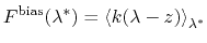
CZAR estimator of the free energy
The corrected z-averaged restraint (CZAR) estimator
is described in detail in reference [57].
It is computed automatically in eABF simulations,
regardless of the number of colvars involved.
Note that ABF may also be applied on a combination of extended and non-extended
colvars; in that case, CZAR still provides an unbiased estimate of the free energy gradient.
CZAR estimates the free energy gradient as:
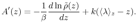 |
(55) |
where
is the colvar,
is the extended variable harmonically
coupled to  with a force constant
, and
with a force constant
, and
 is the observed
distribution (histogram) of
, affected by the eABF bias.
is the observed
distribution (histogram) of
, affected by the eABF bias.
Parameters for the CZAR estimator are:
Similar to ABF, the CZAR estimator produces two output files in multicolumn text format:
- outputName.czar.grad: current estimate of the free energy gradient (grid),
in multicolumn;
- outputName.czar.pmf: only for one-dimensional calculations, integrated
free energy profile or PMF.
The sampling histogram associated with the CZAR estimator is the
-histogram,
which is written in the file outputName.zcount.
Zheng/Yang estimator of the free energy
This feature has been contributed to NAMD by the following authors:
Haohao Fu and Christophe Chipot
Laboratoire International Associé
Centre National de la Recherche Scientifique et University of Illinois at Urbana-Champaign,
Unité Mixte de Recherche No. 7565, Université de Lorraine,
B.P. 70239, 54506 Vand uvre-lès-Nancy cedex, France
© 2016, CENTRE NATIONAL DE LA RECHERCHE SCIENTIFIQUE
This implementation is fully documented in [32].
The Zheng and Yang estimator [110] is based on Umbrella Integration [48].
The free energy gradient is estimated as :
![$\displaystyle A'(\xi^*) = \frac{\displaystyle \sum_{\lambda} N(\xi^*, \lambda) ...
...- k (\xi^* - \lambda) \right]} {\displaystyle \sum_{\lambda} N(\xi^*, \lambda)}$](img425.png) |
(56) |
where
is the colvar,
is the extended variable harmonically
coupled to
with a force constant
,
 is the number of samples collected in a
 bin, which is assumed to be a Gaussian function
of
with mean
bin, which is assumed to be a Gaussian function
of
with mean
 and standard deviation
 .
.
The estimator is enabled through the following option:
- UIestimator
Calculate UI estimator of the free energy?
Context: abf
Acceptable Values: boolean
Default Value: no
Description: This option is only available when ABF is performed on extended-Lagrangian colvars.
When enabled, it triggers calculation of the free energy following the UI estimator.
The eABF algorithm can be associated with a multiple-walker strategy [68,25] (9.5.1).
To run a multiple-replica eABF simulation, start a multiple-replica
NAMD run (option +replicas) and set shared on in the Colvars config file to enable
the multiple-walker ABF algorithm.
It should be noted that in contrast with classical MW-ABF simulations,
the output files of an MW-eABF simulation only show the free energy estimate of
the corresponding replica.
One can merge the results, using
./eabf.tcl -mergemwabf [merged_filename] [eabf_output1] [eabf_output2] ...,
e.g.,
./eabf.tcl -mergemwabf merge.eabf eabf.0.UI eabf.1.UI eabf.2.UI eabf.3.UI.
If one runs an ABF-based calculation, breaking the reaction pathway
into several non-overlapping windows, one can use
./eabf.tcl -mergesplitwindow [merged_fileprefix] [eabf_output] [eabf_output2] ...
to merge the data accrued in these non-overlapping windows.
This option can be utilized in both eABF and classical ABF simulations, e.g.,
./eabf.tcl -mergesplitwindow merge window0.czar window1.czar window2.czar window3.czar,
./eabf.tcl -mergesplitwindow merge window0.UI window1.UI window2.UI window3.UI or
./eabf.tcl -mergesplitwindow merge abf0 abf1 abf2 abf3.
Metadynamics
The metadynamics method uses a history-dependent potential [54] that generalizes to any type of colvars the conformational flooding [36] and local elevation [44] methods, originally formulated to use as colvars the principal components of a covariance matrix or a set of dihedral angles, respectively.
The metadynamics potential on the colvars
 is defined as:
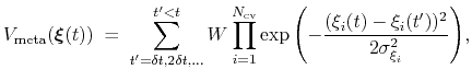 |
(57) |
where
 is the history-dependent potential acting on the current values of the colvars
, and depends only parametrically on the previous values of the colvars.
is constructed as a sum of
is the history-dependent potential acting on the current values of the colvars
, and depends only parametrically on the previous values of the colvars.
is constructed as a sum of
 -dimensional repulsive Gaussian ``hills'', whose height is a chosen energy constant
  , and whose centers are the previously explored configurations
 .
.
During the simulation, the system evolves towards the nearest minimum of the ``effective'' potential of mean force
 , which is the sum of the ``real'' underlying potential of mean force
 and the the metadynamics potential,
 .
Therefore, at any given time the probability of observing the configuration
.
Therefore, at any given time the probability of observing the configuration
 is proportional to
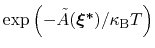 : this is also the probability that a new Gaussian ``hill'' is added at that configuration.
If the simulation is run for a sufficiently long time, each local minimum is canceled out by the sum of the Gaussian ``hills''.
At that stage the ``effective'' potential of mean force
is constant, and
: this is also the probability that a new Gaussian ``hill'' is added at that configuration.
If the simulation is run for a sufficiently long time, each local minimum is canceled out by the sum of the Gaussian ``hills''.
At that stage the ``effective'' potential of mean force
is constant, and
 is an accurate estimator of the ``real'' potential of mean force
, save for an additive constant:
is an accurate estimator of the ``real'' potential of mean force
, save for an additive constant:
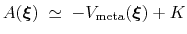 |
(58) |
Assuming that the set of collective variables includes all relevant degrees of freedom, the predicted error of the estimate is a simple function of the correlation times of the colvars
 , and of the user-defined parameters
,
, and of the user-defined parameters
,
 and
and  [16].
In typical applications, a good rule of thumb can be to choose the ratio
[16].
In typical applications, a good rule of thumb can be to choose the ratio
 much smaller than
 , where
 is the longest among
's correlation times:
then dictates the resolution of the calculated PMF.
is the longest among
's correlation times:
then dictates the resolution of the calculated PMF.
Basic syntax
To enable a metadynamics calculation, a metadynamics {...} block must be defined in the Colvars configuration file.
Its mandatory keywords are colvars (see 9.5), which lists all the variables involved, hillWeight (see 9.5.3), which specifies the weight parameter
, and hillWidth (see 9.5.3), which defines the Gaussian width
 as a number of grid points.
Output files
When interpolating grids are enabled (default behavior), the PMF is written by default every colvarsRestartFrequency steps to the file outputName.pmf.
The following two options allow to disable or control this behavior and to track statistical convergence:
Note: when Gaussian hills are deposited near the lowerBoundary (see 9.3.8) or upperBoundary (see 9.3.8) and interpolating grids are used (default behavior), their truncation can give rise to accumulating errors.
In these cases, as a measure of fault-tolerance all Gaussian hills near the boundaries are included in the output state file, and are recalculated analytically whenever the variable falls outside the grid's boundaries.
(Such measure protects the accuracy of the calculation, and can only be disabled by hardLowerBoundary or hardUpperBoundary.)
To avoid gradual loss of performance and growth of the state file, either one of the following solutions is recommended:
- enabling the option expandBoundaries, so that the grid's boundaries are automatically recalculated whenever necessary; the resulting .pmf will have its abscissas expanded accordingly;
- applying a harmonicWalls bias with the wall locations well within the interval delimited by lowerBoundary and upperBoundary.
Performance tuning
The following options control the computational cost of metadynamics calculations, but do not affect results.
Default values are chosen to minimize such cost with no loss of accuracy.
Well-tempered metadynamics
The following options define the configuration for the ``well-tempered'' metadynamics approach [4]:
Multiple-replicas metadynamics
The following options define metadynamics calculations with more than
one replica:
- multipleReplicas
Multiple replicas metadynamics
Context: metadynamics
Acceptable Values: boolean
Default Value: off
Description: If this option is on, multiple (independent) replica of the
same system can be run at the same time, and their hills will be
combined to obtain a single PMF [81]. Replicas are
identified by the value of replicaID. Communication is
done by files: each replica must be able to read the files
created by the others, whose paths are communicated through the file
replicasRegistry. This file, and the files listed in it,
are read every replicaUpdateFrequency steps. Every time
the colvars state file is written
(colvarsRestartFrequency), the file:
``outputName.colvars.name.replicaID.state''
is also written, containing
the state of the metadynamics bias for replicaID. In the
time steps between colvarsRestartFrequency, new hills are
temporarily written to the file:
``outputName.colvars.name.replicaID.hills'',
which serves as communication
buffer. These files are only required for communication, and may be
deleted after a new MD run is started with a different
outputName.
- replicaID
Set the identifier for this replica
Context: metadynamics
Acceptable Values: string
Description: If multipleReplicas is on, this option sets a
unique identifier for this replica. All replicas should use
identical collective variable configurations, except for the value
of this option.
- replicasRegistry
Multiple replicas database file
Context: metadynamics
Acceptable Values: UNIX filename
Default Value: ``name.replica_files.txt''
Description: If multipleReplicas is on, this option sets the
path to the replicas' database file.
- replicaUpdateFrequency
How often hills are communicated between
replicas
Context: metadynamics
Acceptable Values: positive integer
Default Value: newHillFrequency
Description: If multipleReplicas is on, this option sets the
number of steps after which each replica (re)reads the other
replicas' files. The lowest meaningful value of this number is
newHillFrequency. If access to the file system is
significantly affecting the simulation performance, this number can
be increased, at the price of reduced synchronization between
replicas. Values higher than colvarsRestartFrequency may
not improve performance significantly.
- dumpPartialFreeEnergyFile
Periodically write the contribution to the
PMF from this replica
Context: metadynamics
Acceptable Values: boolean
Default Value: on
Description: When multipleReplicas is on, the file
outputName.pmf contains the combined PMF from all
replicas, provided that useGrids is on (default).
Enabling this option produces an additional file
outputName.partial.pmf, which can be useful to
quickly monitor the contribution of each replica to the PMF.
Compatibility and post-processing
The following options may be useful only for applications that go beyond the calculation of a PMF by metadynamics:
- name
Name of this metadynamics instance
Context: metadynamics
Acceptable Values: string
Default Value: ``meta'' + rank number
Description: This option sets the name for this metadynamics instance. While it
is not advisable to use more than one metadynamics instance within
the same simulation, this allows to distinguish each instance from
the others. If there is more than one metadynamics instance, the
name of this bias is included in the metadynamics output file names, such as e.g. the .pmf file.
- keepHills
Write each individual hill to the state
file
Context: metadynamics
Acceptable Values: boolean
Default Value: off
Description: When useGrids and this option are on, all hills
are saved to the state file in their analytic form, alongside their
grids. This makes it possible to later use exact analytic Gaussians
for rebinGrids. To only keep track of the history of the
added hills, writeHillsTrajectory is preferable.
- writeHillsTrajectory
Write a log of new hills
Context: metadynamics
Acceptable Values: boolean
Default Value: off
Description: If this option is on, a logfile is written by the
metadynamics bias, with the name
``outputName.colvars.
name
.hills.traj'', which
can be useful to follow the time series of the hills. When
multipleReplicas is on, its name changes to
``outputName.colvars.
name
.
replicaID
.hills.traj''.
This file can be used to quickly visualize the positions of all
added hills, in case newHillFrequency does not coincide
with colvarsRestartFrequency.
Harmonic restraints
The harmonic biasing method may be used to enforce fixed or moving restraints,
including variants of Steered and Targeted MD. Within energy minimization
runs, it allows for restrained minimization, e.g. to calculate relaxed potential
energy surfaces. In the context of the Colvars module,
harmonic potentials are meant according to their textbook definition:
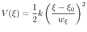 |
(59) |
Note that this differs from harmonic bond and angle potentials in common
force fields, where the factor of one half is typically omitted,
resulting in a non-standard definition of the force constant.
The formula above includes the characteristic length scale  of the colvar
(keyword lowerBoundary (see 9.3.8)) to allow the definition of a multi-dimensional restraint with a unified force constant:
of the colvar
(keyword lowerBoundary (see 9.3.8)) to allow the definition of a multi-dimensional restraint with a unified force constant:
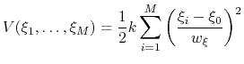 |
(60) |
If one-dimensional or homogeneous multi-dimensional restraints are defined, and there are no other uses for the parameter
, the parameter width can be left at its default value of  .
.
The restraint energy is reported by NAMD under the MISC title.
A harmonic restraint is set up by a harmonic {...}
block, which may contain (in addition to the standard option
colvars) the following keywords:
-
name: see definition of name in sec. 9.5 (biasing and analysis methods)
-
colvars: see definition of colvars in sec. 9.5 (biasing and analysis methods)
-
outputEnergy: see definition of outputEnergy in sec. 9.5 (biasing and analysis methods)
-
writeTIPMF: see definition of writeTIPMF in sec. 9.5 (biasing and analysis methods)
-
writeTISamples: see definition of writeTISamples in sec. 9.5 (biasing and analysis methods)
- forceConstant
Scaled force constant (kcal/mol)
Context: harmonic
Acceptable Values: positive decimal
Default Value: 1.0
Description: This option defines a scaled force constant
for the harmonic potential (eq. 61).
To ensure consistency for multidimensional restraints, it is divided internally by the square of the specific width of each variable (which is 1 by default).
This makes all values effectively dimensionless and of commensurate size.
For instance, setting a scaled force constant of 10 kcal/mol acting on two variables, an angle with a width of 5 degrees and a distance with a width of 0.5 Å, will apply actual force constants of 0.4 kcal/mol degree
 for the angle and 40 kcal/mol/Å
 for the distance.
The values of the actual force constants are always printed when the restraint is defined.
for the distance.
The values of the actual force constants are always printed when the restraint is defined.
- centers
Initial harmonic restraint centers
Context: harmonic
Acceptable Values: space-separated list of colvar values
Description: The centers (equilibrium values) of the restraint,  , are entered here.
The number of values must be the number of requested colvars.
Each value is a decimal number if the corresponding colvar returns
a scalar, a ``(x, y, z)'' triplet if it returns a unit
vector or a vector, and a ``(q0, q1, q2, q3)'' quadruplet
if it returns a rotational quaternion. If a colvar has
periodicities or symmetries, its closest image to the restraint
center is considered when calculating the harmonic potential.
, are entered here.
The number of values must be the number of requested colvars.
Each value is a decimal number if the corresponding colvar returns
a scalar, a ``(x, y, z)'' triplet if it returns a unit
vector or a vector, and a ``(q0, q1, q2, q3)'' quadruplet
if it returns a rotational quaternion. If a colvar has
periodicities or symmetries, its closest image to the restraint
center is considered when calculating the harmonic potential.
Tip: A complex set of restraints can be applied to a system,
by defining several colvars, and applying one or more harmonic
restraints to different groups of colvars. In some cases, dozens of
colvars can be defined, but their value may not be relevant: to
limit the size of the colvars trajectory file, it
may be wise to disable outputValue for such ``ancillary''
variables, and leave it enabled only for ``relevant'' ones.
Moving restraints: steered molecular dynamics
The following options allow to change gradually the centers of the harmonic restraints during a simulations.
When the centers are changed continuously, a steered MD in a collective variable space is carried out.
- targetCenters
Steer the restraint centers towards these
targets
Context: harmonic
Acceptable Values: space-separated list of colvar values
Description: When defined, the current centers will be moved towards
these values during the simulation.
By default, the centers are moved over a total of
targetNumSteps steps by a linear interpolation, in the
spirit of Steered MD.
If targetNumStages is set to a nonzero value, the
change is performed in discrete stages, lasting targetNumSteps
steps each. This second mode may be used to sample successive
windows in the context
of an Umbrella Sampling simulation.
When continuing a simulation
run, the centers specified in the configuration file
colvarsConfig
are overridden by those saved in
the restart file
colvarsInput
.
To perform Steered MD in an arbitrary space of colvars, it is sufficient
to use this option and enable outputAccumulatedWork and/or
outputAppliedForce within each of the colvars involved.
- targetNumSteps
Number of steps for steering
Context: harmonic
Acceptable Values: positive integer
Description: In single-stage (continuous) transformations, defines the number of MD
steps required to move the restraint centers (or force constant)
towards the values specified with targetCenters or
targetForceConstant.
After the target values have been reached, the centers (resp. force
constant) are kept fixed. In multi-stage transformations, this sets the
number of MD steps per stage.
- outputCenters
Write the current centers to the trajectory file
Context: harmonic
Acceptable Values: boolean
Default Value: off
Description: If this option is chosen and colvarsTrajFrequency is not zero, the positions of the restraint centers will be written to the trajectory file during the simulation.
This option allows to conveniently extract the PMF from the colvars trajectory files in a steered MD calculation.
Note on restarting moving restraint simulations: Information
about the current step and stage of a simulation with moving restraints
is stored in the restart file (state file). Thus, such simulations can
be run in several chunks, and restarted directly using the same colvars
configuration file. In case of a restart, the values of parameters such
as targetCenters, targetNumSteps, etc. should not be
changed manually.
Moving restraints: umbrella sampling
The centers of the harmonic restraints can also be changed in discrete stages: in this cases a one-dimensional umbrella sampling simulation is performed.
The sampling windows in simulation are calculated in sequence.
The colvars trajectory file may then be used both to evaluate the correlation times between consecutive windows, and to calculate the frequency distribution of the colvar of interest in each window.
Furthermore, frequency distributions on a predefined grid can be automatically obtained by using the histogram bias (see 9.5.9).
To activate an umbrella sampling simulation, the same keywords as in the previous section can be used, with the addition of the following:
Changing force constant
The force constant of the harmonic restraint may also be changed to equilibrate [29].
- targetForceConstant
Change the force constant towards this value
Context: harmonic
Acceptable Values: positive decimal
Description: When defined, the current forceConstant will be moved towards
this value during the simulation. Time evolution of the force constant
is dictated by the targetForceExponent parameter (see below).
By default, the force constant is changed smoothly over a total of
targetNumSteps steps. This is useful to introduce or
remove restraints in a progressive manner.
If targetNumStages is set to a nonzero value, the
change is performed in discrete stages, lasting targetNumSteps
steps each. This second mode may be used to compute the
conformational free energy change associated with the restraint, within
the FEP or TI formalisms. For convenience, the code provides an estimate
of the free energy derivative for use in TI. A more complete free energy
calculation (particularly with regard to convergence analysis),
while not handled by the Colvars module, can be performed by post-processing
the colvars trajectory, if colvarsTrajFrequency is set to a
suitably small value. It should be noted, however, that restraint
free energy calculations may be handled more efficiently by an
indirect route, through the
determination of a PMF for the restrained coordinate.[29]
- targetForceExponent
Exponent in the time-dependence of the force constant
Context: harmonic
Acceptable Values: decimal equal to or greater than 1.0
Default Value: 1.0
Description: Sets the exponent,  , in the function used to vary the force
constant as a function of time. The force is varied according to a
coupling parameter
, raised to the power
:
, in the function used to vary the force
constant as a function of time. The force is varied according to a
coupling parameter
, raised to the power
:
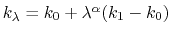 , where
  ,
,
 , and
, and  are the initial, current, and final values
of the force constant. The parameter
evolves linearly from
0 to 1, either smoothly, or in targetNumStages equally spaced
discrete stages, or according to an arbitrary schedule set with
lambdaSchedule.
When the initial value of the force constant is zero,
an exponent greater than 1.0 distributes the effects of introducing the
restraint more smoothly over time than a linear dependence, and
ensures that there is no singularity in the derivative of the
restraint free energy with respect to lambda. A value of 4 has
been found to give good results in some tests.
are the initial, current, and final values
of the force constant. The parameter
evolves linearly from
0 to 1, either smoothly, or in targetNumStages equally spaced
discrete stages, or according to an arbitrary schedule set with
lambdaSchedule.
When the initial value of the force constant is zero,
an exponent greater than 1.0 distributes the effects of introducing the
restraint more smoothly over time than a linear dependence, and
ensures that there is no singularity in the derivative of the
restraint free energy with respect to lambda. A value of 4 has
been found to give good results in some tests.
- targetEquilSteps
Number of steps discarded from TI estimate
Context: harmonic
Acceptable Values: positive integer
Description: Defines the number of steps within each stage that are considered
equilibration and discarded from the restraint free energy derivative
estimate reported reported in the output.
- lambdaSchedule
Schedule of lambda-points for changing force constant
Context: harmonic
Acceptable Values: list of real numbers between 0 and 1
Description: If specified together with targetForceConstant, sets the sequence of
discrete
values that will be used for different stages.
Computing the work of a changing restraint
If the restraint centers or force constant are changed continuosly (targetNumStages undefined) it is possible to record the net work performed by the changing restraint:
- outputAccumulatedWork
Write the accumulated work of the changing restraint to the Colvars trajectory file
Context: harmonic
Acceptable Values: boolean
Default Value: off
Description: If targetCenters or targetForceConstant are defined and this option is enabled, the accumulated work from the beginning of the simulation will be written to the trajectory file (colvarsTrajFrequency must be non-zero).
When the simulation is continued from a state file, the previously accumulated work is included in the integral.
This option allows to conveniently extract the estimated PMF of a steered MD calculation (when targetCenters is used), or of other simulation protocols.
Harmonic wall restraints
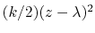
The harmonicWalls {...} bias is closely related to the harmonic bias (see 9.5.4), with the following two differences: (i) instead of a center a lower wall and/or an upper wall are defined, outside of which the bias implements a half-harmonic potential;
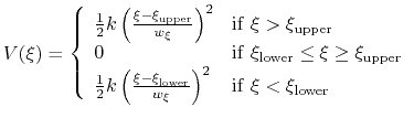 |
(61) |
where
 and
and
 are the lower and upper wall thresholds, respectively; (ii) because an interval between two walls is defined, only scalar variables can be used (but any number of variables can be defined, and the wall bias is intrinsically multi-dimensional).
Note: this bias replaces the keywords lowerWall, lowerWallConstant, upperWall and upperWallConstant defined in the colvar context (see 9.3).
These keywords are still supported, but are deprecated for future uses.
The harmonicWalls bias implements the following options:
Linear restraints
The linear restraint biasing method is used to minimally bias a
simulation. There is generally a unique strength of bias for each CV
center, which means you must know the bias force constant specifically
for the center of the CV. This force constant may be found by using
experiment directed simulation described in
section 9.5.8. Please cite Pitera and Chodera when
using [78].
-
name: see definition of name in sec. 9.5 (biasing and analysis methods)
-
colvars: see definition of colvars in sec. 9.5 (biasing and analysis methods)
-
outputEnergy: see definition of outputEnergy in sec. 9.5 (biasing and analysis methods)
- forceConstant
Scaled force constant (kcal/mol)
Context: linear
Acceptable Values: positive decimal
Default Value: 1.0
Description: This option defines a scaled force constant for the linear bias.
To ensure consistency for multidimensional restraints, it is divided internally by the specific width of each variable (which is 1 by default), so that all variables are effectively dimensionless and of commensurate size.
The values of the actual force constants are always printed when the restraint is defined.
- centers
Initial linear restraint centers
Context: linear
Acceptable Values: space-separated list of colvar values
Description: These are analogous to the centers (see 9.5.4) keyword of the harmonic restraint.
Although they do not affect dynamics, they are here necessary to ensure a well-defined energy for the linear bias.
-
writeTIPMF: see definition of writeTIPMF in sec. 9.5 (biasing and analysis methods)
-
writeTISamples: see definition of writeTISamples in sec. 9.5 (biasing and analysis methods)
-
targetForceConstant: see definition of targetForceConstant in sec. 9.5.4 (Harmonic restraints)
-
targetNumSteps: see definition of targetNumSteps in sec. 9.5.4 (Harmonic restraints)
-
targetForceExponent: see definition of targetForceExponent in sec. 9.5.4 (Harmonic restraints)
-
targetEquilSteps: see definition of targetEquilSteps in sec. 9.5.4 (Harmonic restraints)
-
targetNumStages: see definition of targetNumStages in sec. 9.5.4 (Harmonic restraints)
-
lambdaSchedule: see definition of lambdaSchedule in sec. 9.5.4 (Harmonic restraints)
-
outputAccumulatedWork: see definition of outputAccumulatedWork in sec. 9.5.4 (Harmonic restraints)
Adaptive Linear Bias/Experiment Directed Simulation
Experiment directed simulation applies a linear bias with a changing
force constant. Please cite White and Voth [106] when
using this feature. As opposed to that reference, the force constant here is scaled
by the width corresponding to the biased colvar. In White and
Voth, each force constant is scaled by the colvars set center. The
bias converges to a linear bias, after which it will be the minimal
possible bias. You may also stop the simulation, take the median of
the force constants (ForceConst) found in the colvars trajectory file,
and then apply a linear bias with that constant. All the notes about
units described in sections 9.5.7
and 9.5.4 apply here as well. This is not
a valid simulation of any particular statistical ensemble and is only
an optimization algorithm until the bias has converged.
-
name: see definition of name in sec. 9.5 (biasing and analysis methods)
-
colvars: see definition of colvars in sec. 9.5 (biasing and analysis methods)
- centers
Collective variable centers
Context: alb
Acceptable Values: space-separated list of colvar values
Description: The desired center (equilibrium values) which will be sought during the
adaptive linear biasing.
The number of values must be the number of requested colvars.
Each value is a decimal number if the corresponding colvar returns
a scalar, a ``(x, y, z)'' triplet if it returns a unit
vector or a vector, and a ``q0, q1, q2, q3)'' quadruplet
if it returns a rotational quaternion. If a colvar has
periodicities or symmetries, its closest image to the restraint
center is considered when calculating the linear potential.
- updateFrequency
The duration of updates
Context: alb
Acceptable Values: An integer
Description: This is,  , the number of simulation steps to use for each update to the bias.
This determines how long the system requires to equilibrate
after a change in force constant (
, the number of simulation steps to use for each update to the bias.
This determines how long the system requires to equilibrate
after a change in force constant ( ), how long statistics
are collected for an iteration (
), and how quickly energy is
added to the system (at most,
), how long statistics
are collected for an iteration (
), and how quickly energy is
added to the system (at most,  , where
  is the forceRange). Until the force
constant has converged, the method as described is an
optimization procedure and not an integration of a particular
statistical ensemble. It is important that each step should be
uncorrelated from the last so that iterations are independent.
Therefore,
should be at least twice the autocorrelation time
of the collective variable. The system should also be able to
dissipate energy as fast as
, which can be done by adjusting
thermostat parameters. Practically,
has been tested successfully at
significantly shorter than the autocorrelation time of the
collective variables being biased and still converge correctly.
is the forceRange). Until the force
constant has converged, the method as described is an
optimization procedure and not an integration of a particular
statistical ensemble. It is important that each step should be
uncorrelated from the last so that iterations are independent.
Therefore,
should be at least twice the autocorrelation time
of the collective variable. The system should also be able to
dissipate energy as fast as
, which can be done by adjusting
thermostat parameters. Practically,
has been tested successfully at
significantly shorter than the autocorrelation time of the
collective variables being biased and still converge correctly.
- forceRange
The expected range of the force constant in units of energy
Context: alb
Acceptable Values: A space-separated list of decimal numbers
Default Value: 3 
Description: This is largest magnitude of the force constant which one expects. If this parameter is
too low, the simulation will not converge. If it is too high the
simulation will waste time exploring values that are too
large. A value of 3
has worked well in the systems presented
as a first choice. This parameter is dynamically adjusted over
the course of a simulation. The benefit is that a bad guess for
the forceRange can be corrected. However, this can lead to
large amounts of energy being added over time to the system. To
prevent this dynamic update, add hardForceRange yes
as a parameter
- rateMax
The maximum rate of change of force constant
Context: alb
Acceptable Values: A list of space-separated real numbers
Description: This optional parameter controls
how much energy is added to the system from this bias. Tuning
this separately from the updateFrequency
and forceRange can allow for large bias changes but
with a low rateMax prevents large energy changes that
can lead to instability in the simulation.
Multidimensional histograms
The histogram feature is used to record the distribution of a set of collective
variables in the form of a N-dimensional histogram.
As with any other biasing and analysis method, when a histogram is applied to
an extended-system colvar (9.3.10), it accesses the value
of the fictitious coordinate rather than that of the ``true'' colvar.
A joint histogram of the ``true'' colvar and the fictitious coordinate
may be obtained by specifying the colvar name twice in a row
in the colvars parameter: the first instance will be understood as the
``true'' colvar, and the second, as the fictitious coordinate.
A histogram block may define the following parameters:
-
name: see definition of name in sec. 9.5 (biasing and analysis methods)
-
colvars: see definition of colvars in sec. 9.5 (biasing and analysis methods)
- outputFreq
Frequency (in timesteps) at which the histogram files are refreshed
Context: histogram
Acceptable Values: positive integer
Default Value: colvarsRestartFrequency
Description: The histogram data are written to files at the given time interval.
A value of 0 disables the creation of these files (note: all data to continue a simulation are still included in the state file).
- outputFile
Write the histogram to a file
Context: histogram
Acceptable Values: UNIX filename
Default Value: outputName.
name
.dat
Description: Name of the file containing histogram data (multicolumn format), which is written every outputFreq steps.
For the special case of 2 variables, Gnuplot may be used to visualize this file.
- outputFileDX
Write the histogram to a file
Context: histogram
Acceptable Values: UNIX filename
Default Value: outputName.
name
.dat
Description: Name of the file containing histogram data (OpenDX format), which is written every outputFreq steps.
For the special case of 3 variables, VMD may be used to visualize this file.
- gatherVectorColvars
Treat vector variables as multiple observations of a scalar variable?
Context: histogram
Acceptable Values: UNIX filename
Default Value: off
Description: When this is set to on, the components of a multi-dimensional colvar (e.g. one based on cartesian, distancePairs, or a vector of scalar numbers given by scriptedFunction) are treated as multiple observations of a scalar variable.
This results in the histogram being accumulated multiple times for each simulation step).
When multiple vector variables are included in histogram, these must have the same length because their components are accumulated together.
For example, if
,
and  are three variables of dimensions 5, 5 and 1, respectively, for each iteration 5 triplets
 (
(
 ) are accumulated into a 3-dimensional histogram.
- weights
Treat vector variables as multiple observations of a scalar variable?
Context: histogram
Acceptable Values: list of space-separated decimals
Default Value: all weights equal to 1
Description: When gatherVectorColvars is on, the components of each multi-dimensional colvar are accumulated with a different weight.
For example, if  and
and  are two distinct cartesian variables defined on the same group of atoms, the corresponding 2D histogram can be weighted on a per-atom basis in the definition of histogram.
Grid definition for multidimensional histograms
Like the ABF and metadynamics biases, histogram uses the parameters lowerBoundary, upperBoundary, and width to define its grid.
These values can be overridden if a configuration block histogramGrid { ...} is provided inside the configuration of histogram.
The options supported inside this configuration block are:
- lowerBoundaries
Lower boundaries of the grid
Context: histogramGrid
Acceptable Values: list of space-separated decimals
Description: This option defines the lower boundaries of the grid, overriding any values defined by the lowerBoundary keyword of each colvar.
Note that when gatherVectorColvars is on, each vector variable is automatically treated as a scalar, and a single value should be provided for it.
-
upperBoundaries: analogous to lowerBoundaries
-
widths: analogous to lowerBoundaries
Probability distribution-restraints
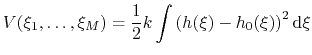
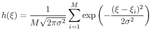
The histogramRestraint bias implements a continuous potential of many variables (or of a single high-dimensional variable) aimed at reproducing a one-dimensional statistical distribution that is provided by the user.
The  variables
 are interpreted as multiple observations of a random variable
with unknown probability distribution.
The potential is minimized when the histogram
are interpreted as multiple observations of a random variable
with unknown probability distribution.
The potential is minimized when the histogram  , estimated as a sum of Gaussian functions centered at
, is equal to the reference histogram
, estimated as a sum of Gaussian functions centered at
, is equal to the reference histogram
 :
:
 |
(62) |
 |
(63) |
When used in combination with a distancePairs multi-dimensional variable, this bias implements the refinement algorithm against ESR/DEER experiments published by Shen et al [88].
This bias behaves similarly to the histogram bias with the gatherVectorColvars option, with the important difference that all variables are gathered, resulting in a one-dimensional histogram.
Future versions will include support for multi-dimensional histograms.
The list of options is as follows:
Defining scripted biases
Rather than using the biasing methods described above, it is possible to apply biases
provided at run time as a Tcl script, in the spirit of TclForces.
- scriptedColvarForces
Enable custom, scripted forces on colvars
Context: global
Acceptable Values: boolean
Default Value: off
Description: If this flag is enabled, a Tcl procedure named calc_colvar_forces
accepting one parameter should be defined by the user. It is executed
at each timestep, with the current step number as parameter, between the
calculation of colvars and the application of bias forces. This procedure
may use the scripting interface (see 9.2.2) to access
the values of colvars and apply forces on them, effectively defining custom
collective variable biases.
Performance of scripted biases
If concurrent computation over multiple threads is available (this is indicated by the message ``SMP parallelism is available.'' printed at initialization time), it is useful to take advantage of the scripting interface to combine many components, all computed in parallel, into a single variable.
The default SMP schedule is the following:
- distribute the computation of all components across available threads;
- on a single thread, collect the results of multi-component variables using polynomial combinations (see 9.3.5), or custom functions (see 9.3.6), or scripted functions (see 9.3.7);
- distribute the computation of all biases across available threads;
- compute on a single thread any scripted biases implemented via the keyword scriptedColvarForces (see 9.5.11).
- communicate on a single thread forces to NAMD.
The following options allow to fine-tune this schedule:
- scriptingAfterBiases
Scripted colvar forces need updated biases?
Context: global
Acceptable Values: boolean
Default Value: on
Description: This flag specifies that the calc_colvar_forces procedure (last step in the list above) is executed only after all biases have been updated (next-to-last step)
For example, this allows using the energy of a restraint bias, or the force applied on a colvar,
to calculate additional scripted forces, such as boundary constraints.
When this flag is set to off, it is assumed that only the values of the variables
(but not the energy of the biases or applied forces) will be used by calc_colvar_forces:
this can be used to schedule the calculation of scripted forces and biases concurrently
to increase performance.
Next: Syntax changes from older
Up: Collective Variable-based Calculations (Colvars)
Previous: Selecting atoms
Contents
Index
http://www.ks.uiuc.edu/Research/namd/