Non-bonded interactions

NAMD has a number of options that control the way that non-bonded interactions are calculated. These options are interrelated and can be quite confusing, so this section attempts to explain the behavior of the non-bonded interactions and how to use these parameters.

Van der Waals interactions

The simplest non-bonded interaction is the van der Waals interaction. In NAMD, van der Waals interactions are always truncated at the cutoff distance, specified by cutoff. The main option that effects van der Waals interactions is the switching parameter. With this option set to on, a smooth switching function will be used to truncate the van der Waals potential energy smoothly at the cutoff distance. A graph of the van der Waals potential with this switching function is shown in Figure 1. If switching is set to off, the van der Waals energy is just abruptly truncated at the cutoff distance, so that energy may not be conserved.

Figure 1: Graph of van der Waals potential with and without the application of the switching function. With the switching function active, the potential is smoothly reduced to 0 at the cutoff distance. Without the switching function, there is a discontinuity where the potential is truncated.

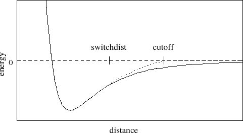The switching function used is based on the X-PLOR switching function. The parameter switchdist specifies the distance at which the switching function should start taking effect to bring the van der Waals potential to 0 smoothly at the cutoff distance. Thus, the value of switchdist must always be less than that of cutoff.

Electrostatic interactions

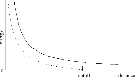
The handling of electrostatics is slightly more complicated due to the incorporation of multiple timestepping for full electrostatic interactions. There are two cases to consider, one where full electrostatics is employed and the other where electrostatics are truncated at a given distance.

First let us consider the latter case, where electrostatics are truncated at the cutoff distance. Using this scheme, all electrostatic interactions beyond a specified distance are ignored, or assumed to be zero. If switching is set to on, rather than having a discontinuity in the potential at the cutoff distance, a shifting function is applied to the electrostatic potential as shown in Figure 2. As this figure shows, the shifting function shifts the entire potential curve so that the curve intersects the x-axis at the cutoff distance. This shifting function is based on the shifting function used by X-PLOR.

Figure 2: Graph showing an electrostatic potential with and without the application of the shifting function.

Next, consider the case where full electrostatics are calculated. In this case, the electrostatic interactions are not truncated at any distance. In this scheme, the cutoff parameter has a slightly different meaning for the electrostatic interactions -- it represents the local interaction distance, or distance within which electrostatic pairs will be directly calculated every timestep. Outside of this distance, interactions will be calculated only periodically. These forces will be applied using a multiple timestep integration scheme as described in Section 7.3.4.

Figure 3: Graph showing an electrostatic potential when full electrostatics are used within NAMD, with one curve portion calculated directly and the other calculated using PME.

Non-bonded force field parameters

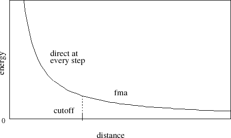• cutoff $<$ local interaction distance common to both electrostatic and van der Waals calculations (Å) $>$
  Acceptable Values: positive decimal
  Description: See Section 5.2 for more information.

• switching $<$ use switching function? $>$
  Acceptable Values: on or off
  Default Value: on
  Description: If switching is specified to be off, then a truncated cutoff is performed. If switching is turned on, then smoothing functions are applied to both the electrostatics and van der Waals forces. For a complete description of the non-bonded force parameters see Section 5.2. If switching is set to on, then switchdist must also be defined.

• vdwForceSwitching $<$ use force switching for VDW? $>$
  Acceptable Values: on or off
  Default Value: off
  Description: If both switching and vdwForceSwitching are set to on, then CHARMM force switching is used for van der Waals forces.

• switchdist $<$ distance at which to activate switching/splitting function for electrostatic and van der Waals calculations (Å) $>$
  Acceptable Values: positive decimal $\leq$ cutoff
  Description: Distance at which the switching function should begin to take effect. This parameter only has meaning if switching is set to on. The value of switchdist must be less than or equal to the value of cutoff, since the switching function is only applied on the range from switchdist to cutoff. For a complete description of the non-bonded force parameters see Section 5.2.

• exclude $<$ non-bonded exclusion policy to use $>$
  Acceptable Values: none, 1-2, 1-3, 1-4, or scaled1-4
  Description: This parameter specifies which pairs of bonded atoms should be excluded from non-bonded interactions. With the value of none, no bonded pairs of atoms will be excluded. With the value of 1-2, all atom pairs that are directly connected via a linear bond will be excluded. With the value of 1-3, all 1-2 pairs will be excluded along with all pairs of atoms that are bonded to a common third atom (i.e., if atom A is bonded to atom B and atom B is bonded to atom C, then the atom pair A-C would be excluded). With the value of 1-4, all 1-3 pairs will be excluded along with all pairs connected by a set of two bonds (i.e., if atom A is bonded to atom B, and atom B is bonded to atom C, and atom C is bonded to atom D, then the atom pair A-D would be excluded). With the value of scaled1-4, all 1-3 pairs are excluded and all pairs that match the 1-4 criteria are modified. The electrostatic interactions for such pairs are modified by the constant factor defined by 1-4scaling. The van der Waals interactions are modified by using the special 1-4 parameters defined in the parameter files. The value of scaled1-4 is necessary to enable the modified 1-4 VDW parameters present in the CHARMM parameter files.

• 1-4scaling $<$ scaling factor for 1-4 electrostatic interactions $>$
  Acceptable Values: 0 $\leq$ decimal $\leq$ 1
  Default Value: 1.0
  Description: Scaling factor for 1-4 electrostatic interactions. This factor is only used when the exclude parameter is set to scaled1-4. In this case, this factor is used to modify the electrostatic interactions between 1-4 atom pairs. If the exclude parameter is set to anything but scaled1-4, this parameter has no effect regardless of its value.

• dielectric $<$ dielectric constant for system $>$
  Acceptable Values: decimal $\geq$ 1.0
  Default Value: 1.0
  Description: Dielectric constant for the system. A value of 1.0 implies no modification of the electrostatic interactions. Any larger value will lessen the electrostatic forces acting in the system.

• nonbondedScaling $<$ scaling factor for nonbonded forces $>$
  Acceptable Values: decimal $\geq$ 0.0
  Default Value: 1.0
  Description: Scaling factor for electrostatic and van der Waals forces. A value of 1.0 implies no modification of the interactions. Any smaller value will lessen the nonbonded forces acting in the system.

• vdwGeometricSigma $<$ use geometric mean to combine L-J sigmas $>$
  Acceptable Values: yes or no
  Default Value: no
  Description: Use geometric mean, as required by OPLS, rather than traditional arithmetic mean when combining Lennard-Jones sigma parameters for different atom types.

• limitdist $<$ maximum distance between pairs for limiting interaction strength(Å) $>$
  Acceptable Values: non-negative decimal
  Default Value: 0.
  Description: The electrostatic and van der Waals potential functions diverge as the distance between two atoms approaches zero. The potential for atoms closer than limitdist is instead treated as $a r^2 + c$ with parameters chosen to match the force and potential at limitdist. This option should primarily be useful for alchemical free energy perturbation calculations, since it makes the process of creating and destroying atoms far less drastic energetically. The larger the value of limitdist the more the maximum force between atoms will be reduced. In order to not alter the other interactions in the simulation, limitdist should be less than the closest approach of any non-bonded pair of atoms; 1.3Å appears to satisfy this for typical simulations but the user is encouraged to experiment. There should be no performance impact from enabling this feature.

• LJcorrection $<$ Apply long-range corrections to the system energy and virial to account for neglected vdW forces? $>$
  Acceptable Values: yes or no
  Default Value: no
  Description: Apply an analytical correction to the reported vdW energy and virial that is equal to the amount lost due to switching and cutoff of the LJ potential. The correction will use the average of vdW parameters for all particles in the system and assume a constant, homogeneous distribution of particles beyond the switching distance. See [89] for details (the equations used in the NAMD implementation are slightly different due to the use of a different switching function). Periodic boundary conditions are required to make use of tail corrections.

PME parameters

PME stands for Particle Mesh Ewald and is an efficient full electrostatics method for use with periodic boundary conditions. None of the parameters should affect energy conservation, although they may affect the accuracy of the results and momentum conservation.

• PME $<$ Use particle mesh Ewald for electrostatics? $>$
  Acceptable Values: yes or no
  Default Value: no
  Description: Turns on particle mesh Ewald.

• PMETolerance $<$ PME direct space tolerance $>$
  Acceptable Values: positive decimal
  Default Value: $10^{-6}$
  Description: Affects the value of the Ewald coefficient and the overall accuracy of the results.

• PMEInterpOrder $<$ PME interpolation order $>$
  Acceptable Values: positive integer
  Default Value: 4 (cubic)
  Description: Charges are interpolated onto the grid and forces are interpolated off using this many points, equal to the order of the interpolation function plus one.

• PMEGridSpacing $<$ maximum space between grid points $>$
  Acceptable Values: positive real
  Description: The grid spacing partially determines the accuracy and efficiency of PME. If any of the grid sizes below are not set, then PMEGridSpacing must be set (recommended value is 1.0 Å) and will be used to calculate them. If a grid size is set, then the grid spacing must be at least PMEGridSpacing (if set, or a very large default of 1.5).

• PMEGridSizeX $<$ number of grid points in x dimension $>$
  Acceptable Values: positive integer
  Description: The grid size partially determines the accuracy and efficiency of PME. For speed, PMEGridSizeX should have only small integer factors (2, 3 and 5).

• PMEGridSizeY $<$ number of grid points in y dimension $>$
  Acceptable Values: positive integer
  Description: The grid size partially determines the accuracy and efficiency of PME. For speed, PMEGridSizeY should have only small integer factors (2, 3 and 5).

• PMEGridSizeZ $<$ number of grid points in z dimension $>$
  Acceptable Values: positive integer
  Description: The grid size partially determines the accuracy and efficiency of PME. For speed, PMEGridSizeZ should have only small integer factors (2, 3 and 5).

• PMEProcessors $<$ processors for FFT and reciprocal sum $>$
  Acceptable Values: positive integer
  Default Value: larger of x and y grid sizes up to all available processors
  Description: For best performance on some systems and machines, it may be necessary to restrict the amount of parallelism used. Experiment with this parameter if your parallel performance is poor when PME is used.

• FFTWEstimate $<$ Use estimates to optimize FFT? $>$
  Acceptable Values: yes or no
  Default Value: no
  Description: Do not optimize FFT based on measurements, but on FFTW rules of thumb. This reduces startup time, but may affect performance.

• FFTWUseWisdom $<$ Use FFTW wisdom archive file? $>$
  Acceptable Values: yes or no
  Default Value: yes
  Description: Try to reduce startup time when possible by reading FFTW ``wisdom'' from a file, and saving wisdom generated by performance measurements to the same file for future use. This will reduce startup time when running the same size PME grid on the same number of processors as a previous run using the same file.

• FFTWWisdomFile $<$ name of file for FFTW wisdom archive $>$
  Acceptable Values: file name
  Default Value: FFTW_NAMD_version_platform.txt
  Description: File where FFTW wisdom is read and saved. If you only run on one platform this may be useful to reduce startup times for all runs. The default is likely sufficient, as it is version and platform specific.

MSM parameters

The multilevel summation method (MSM) [40] is an alternative to PME for calculating full electrostatic interactions. The use of the FFT in PME has two drawbacks: (1) it generally requires the use of periodic boundary conditions, in which the simulation describes an infinite three-dimensional lattice, with each lattice cell containing a copy of the simulated system, and (2) calculation of the FFT becomes a considerable performance bottleneck to the parallel scalability of MD simulations, due to the many-to-many communication pattern employed. MSM avoids the use of the FFT in its calculation, instead employing the nested interpolation in real space of softened pair potentials, which permits in addition to periodic boundary conditions the use of semi-periodic boundaries, in which there is periodicity along just one or two basis vectors, or non-periodic boundaries, in which the simulation is performed in a vacuum. Also, better parallel scaling has been observed with MSM when scaling a sufficiently large system to a large number of processors. See the MSM research web page (http://www.ks.uiuc.edu/Research/msm/) for more information.

In order to use the MSM, one need only specify ``MSM on'' in the configuration file. For production use, we presently recommend using the default ``MSMQuality 0'' ($C^1$ cubic interpolation with $C^2$ Taylor splitting), which has been validated to correctly reproduce the PME results [40]. At this time, we discourage use of the higher order interpolation schemes (Hermite, quintic, etc.), as they are still under development. With cubic interpolation, MSM now gets roughly half the performance of PME. Comparable performance and better scaling for MSM have been observed with the optimizations described in Ref. [40], which will be available shortly.

For now, NAMD's implementation of the MSM does not calculate the long-range electrostatic contribution to the virial, so use with a barostat for constant pressure simulation is inappropriate. (Note that the experiments in Ref. [40] involving constant pressure simulation with MSM made use of a custom version that is incompatible with some other NAMD features, so is not yet available.) The performance of PME is generally still better for smaller systems with smaller processor counts. MSM is the only efficient method in NAMD for calculating full electrostatics for simulations with semi-periodic or non-periodic boundaries.

The periodicity is defined through setting the cell basis vectors appropriately, as discussed in Sec. 7. The cutoff distance, discussed earlier in this section, also determines the splitting distance between the MSM short-range part, calculated exactly, and long-range part, interpolated from the grid hierarchy; this splitting distance is the primary control for accuracy for a given interpolation and splitting, although most simulations will likely want to keep the cutoff set to the CHARMM-prescribed value of 12 Å.

The configuration options specific to MSM are listed below. A simulation employing non-periodic boundaries in one or more dimensions might have atoms that attempt to drift beyond the predetermined extent of the grid. In the case that an atom does drift beyond the grid, the simulation will be halted prematurely with an error message. Several options listed below deal with defining the extent of the grid along non-periodic dimensions beyond what can be automatically determined by the initial coordinates. It is also recommended for non-periodic simulation to configure boundary restraints to contain the atoms, for instance, through Tcl boundary forces in Sec. 8.11.

• MSM $<$ Use multilevel summation method for electrostatics? $>$
  Acceptable Values: yes or no
  Default Value: no
  Description: Turns on multilevel summation method.

• MSMGridSpacing $<$ spacing between finest level grid points (Å) $>$
  Acceptable Values: positive real
  Default Value: 2.5
  Description: The grid spacing determines in part the accuracy and efficiency of MSM. An error versus cost analysis shows that the best tradeoff is setting the grid spacing to a value close to the inter-particle spacing. The default value works well in practice for atomic scale simulation. This value will be exact along non-periodic dimensions. For periodic dimensions, the grid spacing must evenly divide the basis vector length; the actual spacing for a desired grid spacing $h$ is guaranteed to be within the interval $\bigl[ \frac{4}{5} h, \frac{6}{5} h \bigr)$ .

• MSMQuality $<$ select the approximation quality $>$
  Acceptable Values: $0,1,2,3,4$
  Default Value: 0
  Description: This parameter offers a simplified way to select higher order interpolation and splitting for MSM. The available choices are:
  • 0 sets $C^1$ cubic ($p=3$ ) interpolation with $C^2$ Taylor splitting,
  • 1 sets $C^1$ Hermite ($p=4$ ) interpolation with $C^3$ Taylor splitting,
  • 2 sets $C^1$ quintic ($p=5$ ) interpolation with $C^3$ Taylor splitting,
  • 3 sets $C^1$ septic ($p=7$ ) interpolation with $C^4$ Taylor splitting,
  • 4 sets $C^1$ nonic ($p=9$ ) interpolation with $C^5$ Taylor splitting.
  We presently recommend using the default selection, which has been validated to correctly reproduce the PME results [40], and discourage use of the higher order interpolation schemes, as they are still under development. With cubic interpolation, MSM now gets roughly half the performance of PME. Comparable performance and better scaling for MSM have been observed with the optimizations described in Ref. [40], which will be available shortly.

  There is generally a tradeoff between quality and performance. Empirical results show that the $C^1$ interpolation schemes offer a little better accuracy than the alternative interpolation schemes that have greater continuity. Also, better accuracy has been observed by using a splitting function with $C^{\lceil (p+1) / 2 \rceil}$ continuity where $p$ is the order of the interpolant.

• MSMApprox $<$ select the interpolant $>$
  Acceptable Values: $0,1,\dots,7$
  Default Value: 0
  Description: Select the interpolation scheme:
  • 0 sets $C^1$ cubic ($p=3$ ) interpolation,
  • 1 sets $C^1$ quintic ($p=5$ ) interpolation,
  • 2 sets $C^2$ quintic ($p=5$ ) interpolation,
  • 3 sets $C^1$ septic ($p=7$ ) interpolation,
  • 4 sets $C^3$ septic ($p=7$ ) interpolation,
  • 5 sets $C^1$ nonic ($p=9$ ) interpolation,
  • 6 sets $C^4$ nonic ($p=9$ ) interpolation,
  • 7 sets $C^1$ Hermite ($p=4$ ) interpolation.

• MSMSplit $<$ select the splitting $>$
  Acceptable Values: $0,1,\dots,6$
  Default Value: 0
  Description: Select the splitting function:
  • 0 sets $C^2$ Taylor splitting,
  • 1 sets $C^3$ Taylor splitting,
  • 2 sets $C^4$ Taylor splitting,
  • 3 sets $C^5$ Taylor splitting,
  • 4 sets $C^6$ Taylor splitting,
  • 5 sets $C^7$ Taylor splitting,
  • 6 sets $C^8$ Taylor splitting.

• MSMLevels $<$ maximum number of levels $>$
  Acceptable Values: non-negative integer
  Default Value: 0
  Description: Set the maximum number of levels to use in the grid hierarchy. Although setting slightly lower than the default might (or might not) improve performance and/or accuracy for non-periodic simulation, it is generally best to leave this at the default value "0" which will then automatically adjust the levels to the size of the given system.

• MSMPadding $<$ grid padding (Å) $>$
  Acceptable Values: non-negative real
  Default Value: 2.5
  Description: The grid padding applies only to non-periodic dimensions, for which the extent of the grid is automatically determined by the maximum and minimum of the initial coordinates plus the padding value.

• MSMxmin, MSMymin, MSMzmin $<$ minimum x-, y-, z-coordinate (Å) $>$
  Acceptable Values: real
  Description: Set independently the minimum x-, y-, or z-coordinates of the simulation. This parameter is applicable only to non-periodic dimensions. It is useful in conjunction with setting a boundary restraining force with Tcl boundary forces in Sec. 8.11.

• MSMxmax, MSMymax, MSMzmax $<$ maximum x-, y-, z-coordinate (Å) $>$
  Acceptable Values: real
  Description: Set independently the maximum x-, y-, or z-coordinates of the simulation. This parameter is applicable only to non-periodic dimensions. It is useful in conjunction with setting a boundary restraining force with Tcl boundary forces in Sec. 8.11.

• MSMBlockSizeX, MSMBlockSizeY, MSMBlockSizeZ $<$ block size for grid decomposition $>$
  Acceptable Values: positive integer
  Default Value: 8
  Description: Tune parallel performance by adjusting the block size used for parallel domain decomposition of the grid. Recommended to keep the default.

• MSMSerial $<$ Use serial long-range solver? $>$
  Acceptable Values: yes or no
  Default Value: no
  Description: Enable instead the slow serial long-range solver. Intended to be used only for testing and diagnostic purposes.

Full direct parameters

The direct computation of electrostatics is not intended to be used during real calculations, but rather as a testing or comparison measure. Because of the ${\mathcal O}(N^2)$ computational complexity for performing direct calculations, this is much slower than using PME or MSM to compute full electrostatics for large systems. In the case of periodic boundary conditions, the nearest image convention is used rather than a full Ewald sum.

• FullDirect $<$ calculate full electrostatics directly? $>$
  Acceptable Values: yes or no
  Default Value: no
  Description: Specifies whether or not direct computation of full electrostatics should be performed.

Tabulated nonbonded interaction parameters

In order to support coarse grained models and semiconductor force fields, the tabulated energies feature replaces the normal van der Waals potential for specified pairs of atom types with one interpolated from user-supplied energy tables. The electrostatic potential is not altered.

Pairs of atom types to which the modified interactions apply are specified in a CHARMM parameter file by an NBTABLE section consisting of lines with two atom types and a corresponding interaction type name. For example, tabulated interactions for SI-O, O-O, and SI-SI pairs would be specified in a parameter file as:

NBTABLE
SI O SIO
O O OO
SI SI SISI

Each interaction type must correspond to an entry in the energy table file. The table file consists of a header formatted as:

# multiple comment lines
<number_of_tables> <table_spacing (A)> <maximum_distance (A)>

followed by number_of_tables energy tables formatted as:

TYPE <interaction type name>
0 <energy (kcal/mol)> <force (kcal/mol/A)>
<table_spacing> <energy (kcal/mol)> <force (kcal/mol/A)>
<2*table_spacing> <energy (kcal/mol)> <force (kcal/mol/A)>
<3*table_spacing> <energy (kcal/mol)> <force (kcal/mol/A)>
...
<maximum_distance - 3*table_spacing> <energy (kcal/mol)> <force (kcal/mol/A)>
<maximum_distance - 2*table_spacing> <energy (kcal/mol)> <force (kcal/mol/A)>
<maximum_distance - table_spacing> <energy (kcal/mol)> <force (kcal/mol/A)>

The table entry at maximum_distance will match the energy of the previous entry but have a force of zero. The maximum distance must be at least equal to the nonbonded cutoff distance and entries beyond the cutoff distance will be ignored. For the above example with a cutoff of 12 Å the table file could look like:

# parameters for silicon dioxide
3 0.01 14.0
TYPE SIO
0 5.092449e+26 3.055469e+31
0.01 5.092449e+14 3.055469e+17
0.02 7.956951e+12 2.387085e+15
0.03 6.985526e+11 1.397105e+14
...
13.98 0.000000e+00 -0.000000e+00
13.99 0.000000e+00 -0.000000e+00
TYPE OO
0 1.832907e+27 1.099744e+32
0.01 1.832907e+15 1.099744e+18
0.02 2.863917e+13 8.591751e+15
0.03 2.514276e+12 5.028551e+14
...
13.98 0.000000e+00 -0.000000e+00
13.99 0.000000e+00 -0.000000e+00
TYPE SISI
0 0.000000e+00 -0.000000e+00
0.01 0.000000e+00 -0.000000e+00
...
13.98 0.000000e+00 -0.000000e+00
13.99 0.000000e+00 -0.000000e+00

The following three parameters are required for tabulated energies.

• tabulatedEnergies $<$ use tabulated energies $>$
  Acceptable Values: yes or no
  Default Value: no
  Description: Specifies whether or not tabulated energies will be used for van der Waals interactions between specified pairs of atom types.

• tabulatedEnergiesFile $<$ file containing energy table $>$
  Acceptable Values: file name
  Description: Provides one energy table for each interaction type in parameter file. See format above.

• tableInterpType $<$ cubic or linear interpolation $>$
  Acceptable Values: cubic or linear
  Description: Specifies the order for interpolating between energy table entries.