Analysis of Results

Force Analysis for Constant Velocity Pulling

Hopefully your constant velocity SMD simulation has finished successfully and you can proceed with analysing the generated data, specifically the trajectory and the force applied to the SMD atom. In case that you have not succeeded with your simulations we provide the respective files in the subdirectories example-output. For instance, if you do not find a file in the directory common, you should find it in the directory common/example-output.

1

In VMD choose the New Molecule... menu item. Using the Browse... and the Load buttons load the file ubq.psf in the common directory.

2

Now, select with the mouse the molecule (ID 0) in the VMD Main window. Then choose the Load Data Into Molecule... menu item and using the Browse... and the Load buttons load the trajectory file
3-1-pullcv/ubq_ww_pcv.dcd

In the screen you should be able to see the trajectory of the molecular dynamics simulation. By choosing an appropriate representation (e.g. Cartoon) look how the $\beta$ strands behave along the trajectory and how one end of the protein remains fixed while the other one is pulled as you had set it up. (Fig. 20)

Figure: Snapshots of ubiquitin pulling with constant velocity at three different time steps.

After inspecting your trajectory you should extract the force applied to the SMD atom from the NAMD output file:

3

Set your current directory to 3-1-pullcv (type cd 3-1-pullcv).

4

Type the following command: cat ubq_ww_pcv.log $\mid$ awk '{if ($1=="SMD") print $0}'> analysis/smd.dat

This creates a file smd.dat (in the analysis directory) which contains just the SMD information.

In order to obtain the force in the direction of pulling you need to calculate $\vec{f}\cdot\vec{n}$, where $\vec{n}$ is the normalized direction of pulling (in our example it was 0.443, 0.398, 0.803).

5

Change your current directory to analysis (cd analysis) and type the following command:
cat smd.dat $\mid$ awk '{print $1 " " $6*$n_x$ + $7*$n_y$ + $8*$n_z$}'> ft.dat,

where $n_x$, $n_y$ and $n_z$ should be replaced by the values you obtained earlier. You have created a file (ft.dat) that contains force versus time data.(Note that columns 6, 7, and 8 of the file smd.dat are the components of the force)

6

Type xmgrace ft.dat. A plot of force versus time should appear on your screen (Fig. 21).

7

In VMD, look again at the trajectory at different times and try to identify the events that are related to peaks in the force. When you are done close xmgrace.

Figure 21: Force vs Time. Your plot should resemble the graph on the left. The graph on the right was obtained in a simulation where ubiquitin was placed in a water sphere ($\sim$ 26000 atoms) and pulled at 0.5 Å/ps using a time step of 1 femtosecond. The results of this last simulation are in better agreement with actual AFM experiments. The force at the end ($t>400$ps) increases when the protein becomes completely unfolded. The first peak in the force is associated with the breaking of hydrogen bonds between two $\beta$ strands.

Distance Analysis for Constant Force Pulling

1

In VMD, delete the current molecule by choosing the Molecule $\rightarrow$ Delete Molecule menu item.

2

Choose the New Molecule... menu item. Using the Browse... and the Load buttons load the file ubq.psf located in the common directory.

3

Now, select with the mouse the molecule you loaded in the VMD Main window. Then choose the Load Data Into Molecule... menu item and using the Browse... and the Load buttons load the trajectory file
3-2-pullcf/ubq_ww_pcf.dcd. As mentioned before, in case that you have not accomplished the simulation to generate the file, we provide such file at 3-2-pullcf/example-output/ubq_ww_pcf.dcd.

In the OpenGL Display window you will see the trajectory of the constant force pulling simulation.

4

Once the complete trajectory is loaded, use the slider in the VMD Main window to go back to the first frame.

5

Choose the Graphics $\rightarrow$ Representations... menu item. In the Graphical Representations window choose the Cartoon drawing method.

6

Press the Create Rep button in order to create a new representation. In the Selected Atoms text entry delete the word all and type protein and resid 1 76 and name CA.

7

For this representation choose the VDW drawing method. You should be able to see the two C$_{\alpha}$ atoms at the end of your protein as spheres.

8

Hide the first representation by double clicking on it in the Graphical Representations window.

9

Click in the OpenGL Display window and press the key 2 (Shortcut to bond labels). Your cursor should look like a cross. Pick the two spheres displayed. A line linking both atoms should appears with the distance between them.

10

Choose the Graphics $\rightarrow$ Labels... menu item. In the Labels window, choose the label type Bonds. Select the bond displayed, click on the Graph tab and then click on the Graph button. This will create a plot of the distance between these two atoms over time (Fig. 22).

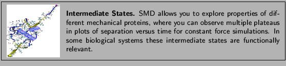
Figure 22: Distance vs Time Steps. Your plot should resemble the graph on the left. The graph on the right was obtained in a simulation where ubiquitin was placed in a water box and pulled from the C-Terminus while keeping the residue K48 fixed. In this case we can observe an intermediate state.

This is the end of the NAMD tutorial. We hope you can now make use of VMD and NAMD in your work.