Next: Non-equilibrium properties of protein
Up: Analysis
Previous: Analysis
Subsections
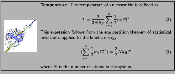
This section contains exercises that will let you analyze properties of a system in equilibrium. The exercises mostly use pre-equilibrated trajectories from different ensembles to calculate properties of the ubiquitin system.
- * 1
- Go to the directory 2-1-rmsd/
You will use a script within VMD that will allow you to compute the average RMSD of each residue in your protein, and assign this value to the B column of the pdb file, which is typically reserved for the temperature factor of each residue.
In the previous unit, you had VMD open with the equilibration trajectory of the ubiquitin cubic system loaded. You will repeat this process:
- * 2
- Launch VMD
- * 3
- You will now load the structure file. First, open the Molecule File Browser from the File
 New Molecule... menu item. Browse for and Load the file ubq_wb.psf in the directory common use the button Up one directory to find it).
- * 4
- The menu at the top of the window should now show 0: ubq_wb.psf. This ensures that the next file that you load will be added to that molecule (molecule ID 0). Now, browse for the file ubq_wb_eq.dcd in the directory 1-3-box/ and click on Load again.
- * 5
- Open the TkCon console by choosing the the Extensions tkcon menu item in VMD.
- * 6
- The script you will use is called residue_rmsd.tcl. In the TkCon window, type:
This command itself does not actually perform any calculations. Instead, it executes the script residue_rmsd.tcl which contains a procedure called rmsd_residue_over_time. Calling this procedure will calculate the average RMSD for each residue you select over all the frames in a trajectory. The procedure is called as:
| rmsd_residue_over_time molsel_resid |
|
where mol is the molecule in VMD that you select (normally, the top molecule), and sel_resid is a list of the residue numbers in that selection. The procedure employs the equations for RMSD shown in Unit 1.
- * 7
- For this example, you will select all the residues in the protein. The list of residue numbers can be obtained by typing in the TkCon:
| set sel_resid [[atomselect top "protein and alpha"] get resid]
|
|
The above command will get the residue numbers of all the  -carbons in the protein (since there is just one and only one -carbon per residue, it is a good option). The command will create a list of residue numbers in the variable $sel_resid.
- * 8
- Call the procedure to calculate the RMSD values of all atoms in the newly created selection:
| rmsd_residue_over_time top $sel_resid |
|
You should see the molecule wiggle as each frame gets aligned to the initial structure. At the end of the calculation, you will get a list of the average RMSD per residue. This data is also printed to the file residue_rmsd.dat.
The procedure also sets the value of the B column of all the atoms of the residues in the selection to the computed RMSD value. You will now color the protein according to this value. You will be able to recognize which residues are free to move more and which ones move less during the equilibration.
In order to use these new values to learn about the mobility of the residues, you will create a representation of the protein colored by B value.
- * 9
- Open the Representations window using the Graphics Representations... menu item.
- * 10
- In the Atom Selection window, type protein. Choose Tube as Drawing Method, and in the Coloring Method drop-down menu, choose Beta. Now, click on the Trajectory tab, and in the Color Scale Data Range, type 0.40 and 1.00. Click the Set button.
You should now see the protein colored according to average RMSD values. The residues displayed in blue are more mobile while the ones in red move less. This is counter intuitive, so you will change the color scale.
- * 11
- Chose the Graphics Colors
 menu item. Choose the Color Scale tab. In the Method pull-down menu, choose BGR. Your figure should now look similar to Fig. 9.
Figure 9:
Ubiquitin colored by the average RMSD per residue. Red denotes more mobile residues, blue residues who moved less during equilibration.
![\begin{figure}\begin{center}
\par\par\latex{
\includegraphics[scale=0.5]{pictures/tut_residue_rmsd}
}
\end{center} \end{figure}](img55.png) |
- * 12
- Look at the RMSD value per residue by typing in a Unix Terminal window (make sure you are in the directory 2-1-rmsd/):
Take a look at the RMSD distribution. You can see regions where a set of residues shows less mobility. Compare with the structural feature of your protein. You will find a correlation between the location of these regions and secondary structure features like helices or  sheets.
- * 1
- Change to the directory 2-2-maxwell/
For this exercise, you will use the last step of the equilibration of ubiquitin. Specifically, you need the file that contains the velocities of every atom in the last frame of this equilibration. The name of the file is ubq_wb_eq.restart.vel, you created it in directory 1-3-box/. We will get the necessary information from this file and the structure file ubq_wb.psf with the help of VMD.
- 2
- Launch VMD.
- 3
- You will now load the structure file. First, open the Molecule File Browser from the File New Molecule... menu item. Browse for and Load the file ubq_wb.psf in the directory common (use the button Up one directory to find it).
- 4
- The menu at the top of the window should now show 0: ubq_wb.psf. This ensures that the next file that you load will be added to that molecule (molecule ID 0). Now, browse for the file ubq_wb_eq.restart.vel in the directory 1-3-box/. This time you need to select the type of file. In the Determine file type: pull-down menu, choose namdbin, and click on Load again.
The molecule you loaded looks terrible! That is because VMD is reading the velocities as if they were coordinates. It does not matter how it looks, because what we want is to make VMD write a useful file: one that contains the masses and velocities for every atom.
- 5
- To execute tcl commands, you will use VMD's TkCon window. Open it by selecting the Extensions tkcon menu item. A console window, the TkCon window, should appear with a prompt. You can now start entering Tcl/Tk commands into it.
- 6
- First, you will create a selection with all the atoms in the system. Do this by typing in the TkCon window:
| set all [atomselect top all] |
|
- 7
- Now, you will open a file energy.dat for writing:
| set fil [open energy.dat w] |
|
- 8
- For each atom in the system, calculate the kinetic energy
 , and write it to a file
| foreach m [$all get mass] v [$all get {x y z}] { |
|
| puts $fil [expr 0.5 * $m *
[vecdot $v $v] ] |
|
| } |
|
- 9
- Close the file:
- 10
- Outside VMD, take a look at your new energy.dat file. You can do this by typing in a Unix Terminal window (make sure you are in the proper directory, i.e. use the same Unix Terminal window from where you launched VMD):
It should look something like:
| 0.39707419313 |
|
| 0.391385065921 |
|
| ... |
|
- 11
- Quit nedit and VMD.
- * 12
- If you chose not to go through the steps above, there is a VMD script that reproduces them and will create the file energy.dat. In a Unix Terminal Window, type:
| vmd -dispdev text -e get_energy.tcl
|
|
This will run VMD in text mode, source the script get_energy.tcl, and produce the energy.dat file.
You now have a file of raw data that you can use to fit the obtained energy distribution to the Maxwell-Boltzmann distribution. You can obtain the temperature of the distribution from that fit. In the rest of this section, we will show how to do this with the 2-D graphics package xmgrace. If you are more familiar with another tool, you may use it instead.
- * 13
- In a Unix Terminal window, type xmgrace.
- * 14
- Once you see the xmgrace window, choose the Data Import ASCII menu item. Select the file energy.dat. Click on the OK button. You should see a black trace. This is the raw data. You can now close the Read sets window.
- * 15
- To look at the distribution of points, you will make a histogram of this data. Choose the Data Transformations Histograms... menu item. In the Source Set window, click on the first line, in order to make a histogram of the data you just loaded.
- * 16
- Click on the Normalize option, and fill in Start: 0, Stop at: 10, and # of bins: 100. Click Apply.
- * 17
- You have created a plot, but you cannot see it yet. Use the right button of your mouse to click on the first set (in the Source Set window). Click on Hide. Now, go to the Main window and click on the button labeled AS, that will resize the plot to fit the existing values. This is your distribution of energies.
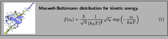
Figure 10:
Maxwell-Boltzmann distribution for kinetic energies.
![\begin{figure}\begin{center}
\par\par\latex{
\includegraphics[scale=0.5]{pictures/tut_unit02_mboltz}
}
\end{center} \end{figure}](img58.png) |
Now, you will fit a Maxwell-Boltzmann distribution to this plot and find out the temperature that the distribution corresponds to. (Hopefully, the temperature you wanted to have in your simulation!)
- * 18
- Choose the Data Transformations Non-linear curve fitting... menu item. In the Source Set window, click on the last line, which corresponds to the histogram you created.
- * 19
- In the Main tab, type in the Formula window:
y = (2/ sqrt(Pi * a0 3 )) * sqrt(x) * exp (-x / a0) 3 )) * sqrt(x) * exp (-x / a0)
|
|
This will fit the curve and get a fit for the parameter a0, which corresponds to  in units of kcal/mol. (These are the energy units that NAMD uses)
- * 20
- In the Parameters drop-down menu, choose 1. Fill-in forms will appear below. You can give an initial value to A0, so that the iterations will look for a value in the vicinity of your initial guess. In the A0 window, type 0.6, which in kcal/mol corresponds to a temperature of
 .
.
- * 21
- Click on the Apply button. This will open a window with the new value for a0, as well as some statistical measures, including the Correlation Coefficient, which is a measure of the fit (better fit as it approaches 1). You can click on the Apply button of the Non-linear fit window several times to obtain a better fit.
- * 22
- The value of a0 you obtained corresponds to . Obtain the temperature
 for this distribution with
 . Your result is hopefully close to
  K!
K!
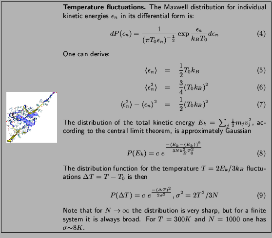
The deviation from your value and the expected one is due to the poor sampling as well as to the finite size of the protein; the latter implies that temperature can be ``measured'' only with an accuracy of about  even in case of perfect sampling.
You will look at the kinetic energy and all internal energies: bonded (bonds, angles and dihedrals) and non-bonded (electrostatic, van der Waals). You should remember that molecular dynamics treats bonds, angles, dihedrals and impropers as harmonic oscillators. You will determine the values of these energies at different temperatures, and find their dependence on this parameter.
To get values over a range of temperatures, you need to look at the output of several simulations, with the same conditions but different temperature. You were provided with a sample configuration file energies.conf for temperature  K. The content of the file is the same as the equilibration configuration file you ran before, except that this time it will have a different value for the temperature. You were assigned a temperature according to your last name.
- * 1
- Go to the directory 2-3-energies/
- * 2
- Using a web browser, go to www.ks.uiuc.edu/
 villa/energies.html and find out which temperature you should simulate.
You need to change the temperature in the script for the temperature you were asked to simulate.
- * 3
- Open a text editor by typing in a Unix Terminal window:
- * 4
- Change the line of the script that contains the value for the temperature by putting your value in there:
| set temperature your_temperature
|
|
When your job simulation is completed, you will need to get the average value of the energies at
 . As you saw, the output file from NAMD has a lot of information. A script called namdstats does all the work for you! The usage of namdstats is:
| namdstats [from first][to last] file
|
|
which calculates the average for all output variables in file from frame first to frame last.
- * 5
- Run namdstats for your output file:
| namdstats from 101 energies.log
|
|
Running from frame 101 will avoid the initial energy and the minimization entries (100).
- * 6
- Go again to www.ks.uiuc.edu/villa/energies.html and follow the link for inputting your values. When everyone else is done, we'll show you a plot of the dependence of the energies on temperature. See what you can learn about it from the result.
- 1
- Go to the directory 2-4-temp/
For this exercise, you need a simulation that is long enough to samle well the quantity of interest, here the fluctuations in kinetic energy, and hence in the temperature. Instead of doing such a simulation yourself, we recommend that you use the provided file ubq-nve.log. However, if you choose to run your own simulation, you can find all the necessary files and instructions below. We recommend you to read the whole section even if you don't perform the simulations.
The simulation is performed in the microcanonical ensemble (NVE, i.e., constant N, V and E). The configuration file provided to start the NAMD run is called ubq-nve.conf. The main features of this configuration file are:
- The simulation takes the restart files from the sphere equilibration simulation performed in Unit 1. The files are located in directory 1-2-sphere/ and are named ubq_ws, i.e., ubq_ws.restart.vel, etc.
- The initial temperature is determined by the velocity restart file as shown in equation above. this initial temperature corresponds to K
- The time step is 2 fs; with rigidBonds turned on, this time step is acceptable.
- The simulation will run for 1 ns.
- * 2
- You need to obtain the data for the temperature from the log file. For this you will use a script called namddat. Do this by typing:
Your data is now in data.dat.
In order to plot the data, you can use xmgrace. You need to remove the line with the title as well as the first line of data, that corresponds to the initial temperature T=0.
- * 3
- Do this using, e.g., nedit:
Remove the first line, save the file as temp.dat and quit nedit. The file temp.dat can now be read by xmgrace and plotted.
- * 4
- Open xmgrace.
- * 5
- Choose the Data Import ASCII menu item. Select the file temp.dat You should see a black trace. This is a plot of the temperature over time.
- * 6
- To look at the distribution of points, you will make a histogram with this data. Choose the Data Transformations Histograms... menu item. In the Source Set window, click on the first line, in order to make a histogram of the data you just loaded.
- * 7
- Click on the Normalize option, and fill in Start: 220, Stop at: 250, and # of bins 100. Click Apply.
- * 8
- You created a plot, but you cannot see it yet. Use the right button of your mouse to click on the first set (in the Source Set window). Click on Hide. Now, go to the Main window and click on the button labeled AS, that will resize the plot to fit the existing values. This is your distribution of temperatures.
Does this distribution look any familiar? Your distribution should look like a Gaussian distribution.
- * 9
- You will now fit your distribution to a normal distribution. For this, you will use the Non-linear curve fitting feature of xmgrace.
- * 10
- Choose the Data Transformations Non-linear curve fitting... menu item. In the Source Set window, click on the last line, which corresponds to the histogram you created.
- * 11
- In the Main tab, type in the Formula window:
y= a0 * exp(-(x-a1)2/a2)
- * 12
- In the Parameters drop-down menu, choose 3. Fill-in frames will appear below. Give A0 an initial value of 1, A1 an initial value of 235 (you can see that the center of the Gaussian is around that value), and A2 a value of 2. Click several times on the Apply, to get a better fit.
This will fit the curve and get values for the parameters a0, a1 and a2, where a0 is a normalization constant, a1 the average temperature, and a2 is  .
.
Figure 11:
Fluctuation of Temperature
![\begin{figure}\begin{center}
\par\par\latex{
\includegraphics[scale=0.5]{pictures/tut_unit02_temp}
}
\end{center} \end{figure}](img76.png) |
The window that appeared contains the new value of the parameters, as well as some statistical measures, including the Correlation Coefficient, which is a measure of the fit.
- * 13
- Compare the average value of the temperature obtained by this method with the one you would obtain using namdstats by typing in a Unix Terminal window:
- * 14
- Now, look at the deviation
 which can be calculated from your data. Note how it is dependent on the size of the system!
Take home message: You may note from this example that single proteins, on the one hand, behave like infinite thermodynamic ensembles, reproducing the respective mean temperature; and, on the other hand, they show signs of their finiteness, i.e. temperature fluctuations. In general, it is interesting to note that the velocities of the atoms and, therefore, the kinetic energy of the protein serves as its thermometer!
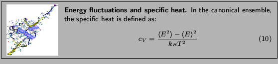
Specific heat is an important property of thermodynamic systems. It is the amount of heat needed to raise the temperature of an object per degree of temperature increase per unit mass, and a sensitive measure of the degree of order in a system. (Near a bistable point, the specific heat becomes large.)
For this exercise, you need to carry out a long simulation in the NVT (canonical) ensemble that samples sufficiently the averages
 and
and
 that arise in the definition of
  . To produce the data for the total energy of the molecule over time, you need to work through the steps presented below. This exercise is long and computationally intensive. We strongly recommend that you work only through the steps marked with *, that correspond to the analysis of the data. Nevertheless, we encourage you to read through the whole method since it will provide you with tools for future analysis.
- * 1
- Change to the directory 2-5-spec_heat/
In order to produce an NVT run, you will restart the equilibration you performed in Unit 1 for the water sphere. All necessary files are present in your directory.
You have now an equilibration run of ubiquitin in the NVT ensemble, and you want to look at the fluctuation in the energy of ubiquitin. The problem is that in order to calculate the specific heat for the protein only (as opposed to the whole system), you need the total energies for the atoms in the protein only, and the NAMD output for the run you just performed contains the energies for all atoms in the system.
You would like NAMD to write the energies for only a part of the system. This feature is currently available in NAMD only for interaction energies between two parts of a system. A way to accomplish this would be to have a system with the protein only, but it does not make sense to equilibrate the protein in this way. However, using a trick, you can make NAMD write the energies for the protein only given the equilibration you already performed.
You will first create a dcd with the protein only. For this, you will use a VMD script called mk_protein_dcd.tcl. This script writes a pdb for each frame of the trajectory, then loads all the pdb files, and writes a dcd file.
- 2
- Run this script in the text mode of VMD:
| vmd -dispdev text -e mk_protein_dcd.tcl
|
|
Note that this script will take a long time to execute!
Now that you have a dcd file for the protein only, you will use the following trick: for each frame of your pre-equilibrated trajectory, start a NAMD simulation that will run for 0 time steps taking the coordinates from the dcd. This will make NAMD write the energies for every frame on the dcd in the output file.
The configuration file for running NAMD in this setup is ubq-get-energy.conf. The way NAMD loops over all frames in the trajectory, taking the coordinates from the current frame and running for 0 time steps is included in this file:
| # runs 0 time steps for each frame in the dcd |
|
| # opens the dcd file to read the coordinates |
|
| coorfile open dcd ubq-nvt.dcd |
|
| set i 0 |
|
| while { ![coorfile read] } { |
|
| incr i |
|
| firsttimestep $i |
|
| run 0 |
|
| } |
|
| coorfile close |
|
Now you have a log file with the energy of the protein. You need to retrieve the values for the total energy and put them into a file:
- * 3
- Use namddat to get TOTAL:
| namddat TOTAL ubq-get-energy.log
|
|
Now that you have a data file data.dat with the energy of the protein over time, you can calculate the energy fluctuation. For this you need:
- * 4
- The average energy, which you can get by using the awk script average.awk (You can use namdstats too) In a Unix Terminal window type:
awk -f average.awk data.dat
- * 5
- The average squared energy, which you can get by using the awk script squared-average.awk:
awk -f squared-average.awk data.dat
- * 6
- Calculate the specific heat for ubiquitin using the equation provided, with
and K. What is your result? Try to convert your results to units of specific heat used everyday, i.e.,
 using the conversion factor
 . Note that this units correspond to the specific heat per unit mass. You calculated the fluctuation in the energy of the whole protein, so you must take into account the mass of your protein by dividing your obtained value by
 . Compare with some specific heats that are given to you in the table below.
| Substance |
Specific Heat |
| |
|
| Human Body(average) |
3470 |
| Wood |
1700 |
| Water |
4180 |
| Alcohol |
2400 |
| Ice |
2100 |
| Gold |
130 |
| Strawberries |
3890 |

Next: Non-equilibrium properties of protein
Up: Analysis
Previous: Analysis
namd@ks.uiuc.edu
![\framebox[\textwidth]{
\begin{minipage}[r]{0.9\textwidth}
\noindent{\textbf{Ob...
...he protein with the residues colored according to this value.}
\end{minipage} }](img51.png)
![\framebox[\textwidth]{
\begin{minipage}{.2\textwidth}
\includegraphics[width=2...
...want to show a property of the system that you have computed.}
\end{minipage} }](img53.png)
![\framebox[\textwidth]{
\begin{minipage}[r]{0.9\textwidth}
\noindent{\textbf{Ob...
...esponds to the Maxwell distribution for a given temperature. }
\end{minipage} }](img56.png)
![\framebox[\textwidth]{
\begin{minipage}[r]{0.9\textwidth}
\noindent{\textbf{Ob...
...e different internal energies) as a function of temperature. }
\end{minipage} }](img67.png)

![\framebox[\textwidth]{
\begin{minipage}[r]{0.9\textwidth}
\noindent{\textbf{Ob...
...in an NVE ensemble, and analyze the temperature distribution.}
\end{minipage} }](img72.png)