Next: Harmonic restraints
Up: Biasing and analysis methods
Previous: Extended-system Adaptive Biasing Force
Contents
Index
Subsections
The metadynamics method uses a history-dependent potential [67] that generalizes to any type of colvars the conformational flooding [68] and local elevation [69] methods, originally formulated to use as colvars the principal components of a covariance matrix or a set of dihedral angles, respectively.
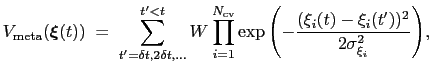
The metadynamics potential on the colvars
 is defined as:
 |
(13.29) |
where
 is the history-dependent potential acting on the current values of the colvars
 , and depends only parametrically on the previous values of the colvars.
is constructed as a sum of
, and depends only parametrically on the previous values of the colvars.
is constructed as a sum of
 -dimensional repulsive Gaussian ``hills'', whose height is a chosen energy constant
  , and whose centers are the previously explored configurations
 .
.
During the simulation, the system evolves towards the nearest minimum of the ``effective'' potential of mean force
 , which is the sum of the ``real'' underlying potential of mean force
 and the the metadynamics potential,
 .
Therefore, at any given time the probability of observing the configuration
.
Therefore, at any given time the probability of observing the configuration
 is proportional to
 : this is also the probability that a new Gaussian ``hill'' is added at that configuration.
If the simulation is run for a sufficiently long time, each local minimum is canceled out by the sum of the Gaussian ``hills''.
At that stage the ``effective'' potential of mean force
is constant, and
: this is also the probability that a new Gaussian ``hill'' is added at that configuration.
If the simulation is run for a sufficiently long time, each local minimum is canceled out by the sum of the Gaussian ``hills''.
At that stage the ``effective'' potential of mean force
is constant, and
 is an estimator of the ``real'' potential of mean force
, save for an additive constant:
is an estimator of the ``real'' potential of mean force
, save for an additive constant:
 |
(13.30) |
Such estimate of the free energy can be provided by enabling writeFreeEnergyFile.
Assuming that the set of collective variables includes all relevant degrees of freedom, the predicted error of the estimate is a simple function of the correlation times of the colvars
 , and of the user-defined parameters
,
, and of the user-defined parameters
,
 and
and  [70].
In typical applications, a good rule of thumb can be to choose the ratio
[70].
In typical applications, a good rule of thumb can be to choose the ratio
 much smaller than
 , where
 is the longest among
's correlation times:
then dictates the resolution of the calculated PMF.
is the longest among
's correlation times:
then dictates the resolution of the calculated PMF.
If the metadynamics parameters are chosen correctly, after an equilibration time,  , the estimator provided
by eq. 13.31 oscillates on time around the ``real'' free energy, thereby a better estimate of the latter can be obtained as the time average of the bias potential after
[71,72]:
, the estimator provided
by eq. 13.31 oscillates on time around the ``real'' free energy, thereby a better estimate of the latter can be obtained as the time average of the bias potential after
[71,72]:
 |
(13.31) |
where
is the time after which the bias potential grows (approximately) evenly during the simulation and  is the total simulation time. The free energy calculated according to eq. 13.32 can thus be obtained averaging on time mutiple time-dependent free energy estimates, that can be printed out through the keyword keepFreeEnergyFiles. An alternative is to obtain the free energy profiles by summing the hills added during the simulation; the hills trajectory can be printed out by enabling the option writeHillsTrajectory.
In typical scenarios the Gaussian hills of a metadynamics potential are interpolated and summed together onto a grid, which is much more efficient than computing each hill independently at every step (the keyword useGrids is on by default).
This numerical approximation typically yields neglibile errors in the resulting PMF [48].
However, due to the finite thickness of the Gaussian function, the metadynamics potential would suddenly vanish each time a variable exceeds its grid boundaries.
To avoid such discontinuity the Colvars metadynamics code will keep an explicit copy of each hill that straddles a grid's boundary, and will use it to compute metadynamics forces outside the grid.
This measure is taken to protect the accuracy and stability of a metadynamics simulation, except in cases of ``natural'' boundaries (for example, the ![$ [0:180]$](img159.png) interval of an angle colvar) or when the flags hardLowerBoundary and hardUpperBoundary are explicitly set by the user.
Unfortunately, processing explicit hills alongside the potential and force grids could easily become inefficient, slowing down the simulation and increasing the state file's size.
interval of an angle colvar) or when the flags hardLowerBoundary and hardUpperBoundary are explicitly set by the user.
Unfortunately, processing explicit hills alongside the potential and force grids could easily become inefficient, slowing down the simulation and increasing the state file's size.
In general, it is a good idea to define a repulsive potential to avoid hills from coming too close to the grid's boundaries, for example as a harmonicWalls restraint (see ![[*]](crossref.png) ).
).
Example: Using harmonic walls to protect the grid's boundaries.
colvar {
name r
distance { ... }
upperBoundary 15.0
width 0.2
}
metadynamics {
name meta_r
colvars r
hillWeight 0.001
hillWidth 2.0
}
harmonicWalls {
name wall_r
colvars r
upperWalls 13.0
upperWallConstant 2.0
}
In the colvar r, the distance function used has a lowerBoundary automatically set to 0 Å by default, thus the keyword lowerBoundary itself is not mandatory and hardLowerBoundary is set to yes internally.
However, upperBoundary does not have such a ``natural'' choice of value.
The metadynamics potential meta_r will individually process any hill whose center is too close to the upperBoundary, more precisely within fewer grid points than 6 times the Gaussian  parameter plus one.
It goes without saying that if the colvar r represents a distance between two freely-moving molecules, it will cross this ``threshold'' rather frequently.
parameter plus one.
It goes without saying that if the colvar r represents a distance between two freely-moving molecules, it will cross this ``threshold'' rather frequently.
In this example, where the value of hillWidth ( ) amounts to 2 grid points, the threshold is 6+1 = 7 grid points away from upperBoundary.
In explicit units, the width of
) amounts to 2 grid points, the threshold is 6+1 = 7 grid points away from upperBoundary.
In explicit units, the width of  is
is  0.2 Å, and the threshold is 15.0 - 7
 0.2 = 13.6 Å.
The wall_r restraint included in the example prevents this: the position of its upperWall is 13 Å, i.e. 3 grid points below the buffer's threshold (13.6 Å).
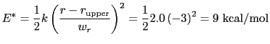
For the chosen value of upperWallConstant, the energy of the wall_r bias at r =
 = 13.6 Å is:
which results in a relative probability
 that r crosses the threshold.
The probability that r exceeds upperBoundary, which is further away, has also become vanishingly small.
At that point, you may want to set hardUpperBoundary to yes for r, and let meta_r know that no special treatment near the grid's boundaries will be needed.
that r crosses the threshold.
The probability that r exceeds upperBoundary, which is further away, has also become vanishingly small.
At that point, you may want to set hardUpperBoundary to yes for r, and let meta_r know that no special treatment near the grid's boundaries will be needed.
What is the impact of the wall restraint onto the PMF? Not a very complicated one: the PMF reconstructed by metadynamics will simply show a sharp increase in free-energy where the wall potential kicks in (r  13 Å).
You may then choose between using the PMF only up until that point and discard the rest, or subtracting the energy of the harmonicWalls restraint from the PMF itself.
Keep in mind, however, that the statistical convergence of metadynamics may be less accurate where the wall potential is strong.
13 Å).
You may then choose between using the PMF only up until that point and discard the rest, or subtracting the energy of the harmonicWalls restraint from the PMF itself.
Keep in mind, however, that the statistical convergence of metadynamics may be less accurate where the wall potential is strong.
In summary, although it would be simpler to set the wall's position upperWall and the grid's boundary upperBoundary to the same number, the finite width of the Gaussian hills calls for setting the former strictly within the latter.
To enable a metadynamics calculation, a metadynamics {...} block must be defined in the Colvars configuration file.
Its mandatory keywords are colvars, the variables involved, hillWeight, the weight parameter
, and the widths
of the Gaussian hills in each dimension given by the single dimensionless parameter hillWidth, or more explicitly by the gaussianSigmas.
-
name: see definition of name (biasing and analysis methods)
-
colvars: see definition of colvars (biasing and analysis methods)
-
outputEnergy: see definition of outputEnergy (biasing and analysis methods)
-
outputFreq: see definition of outputFreq (biasing and analysis methods)
-
writeTIPMF: see definition of writeTIPMF (biasing and analysis methods)
-
writeTISamples: see definition of writeTISamples (biasing and analysis methods)
-
stepZeroData: see definition of stepZeroData (biasing and analysis methods)
-
hillWeight
 Height of each hill (kcal/mol)
Context: metadynamics
Acceptable values: positive decimal
Description: This option sets the height
of the Gaussian hills that are added during this run.
Lower values provide more accurate sampling of the system's degrees of freedom at the price of longer simulation times to complete a PMF calculation based on metadynamics.
-
hillWidth
Width
of a Gaussian hill, measured in number of grid points
Context: metadynamics
Acceptable values: positive decimal
Description: This keyword sets the Gaussian width
 for all colvars, expressed in number of grid points, with the grid spacing along each colvar
  determined by the respective value of width.
Values between 1 and 3 are recommended for this option: smaller numbers will fail to adequately interpolate each Gaussian function [48], while larger values may be unable to account for steep free-energy gradients.
The values of each half-width
in the physical units of
determined by the respective value of width.
Values between 1 and 3 are recommended for this option: smaller numbers will fail to adequately interpolate each Gaussian function [48], while larger values may be unable to account for steep free-energy gradients.
The values of each half-width
in the physical units of  are also printed by VMD at initialization time; alternatively, they may be set explicitly via gaussianSigmas.
-
gaussianSigmas
Half-widths
of the Gaussian hill (one for each colvar)
Context: metadynamics
Acceptable values: space-separated list of decimals
Description: This option sets the parameters
 of the Gaussian hills along each colvar
  , expressed in the same unit of
.
No restrictions are placed on each value, but a warning will be printed if useGrids is on and the Gaussian width
, expressed in the same unit of
.
No restrictions are placed on each value, but a warning will be printed if useGrids is on and the Gaussian width
 is smaller than the corresponding grid spacing,
 .
If not given, default values will be computed from the dimensionless number hillWidth.
.
If not given, default values will be computed from the dimensionless number hillWidth.
-
newHillFrequency
Frequency of hill creation
Context: metadynamics
Acceptable values: positive integer
Default value: 1000
Description: This option sets the number of steps after which a new Gaussian hill is added to the metadynamics potential.
The product of this number and the integration time-step defines the parameter
in eq. 13.30.
Higher values provide more accurate statistical sampling, at the price of longer simulation times to complete a PMF calculation.
When analyzing data from a previous simulation in VMD, the metadynamics potential does not need to be updated, and it is useful to set this number to 0.
When interpolating grids are enabled (default behavior), the PMF is written by default every colvarsRestartFrequency steps to the file outputName.pmf in multicolumn text format ().
The following two options allow to disable or control this behavior and to track statistical convergence:
-
writeFreeEnergyFile
Periodically write the PMF for visualization
Context: metadynamics
Acceptable values: boolean
Default value: on
Description: When useGrids and this option are on, the PMF is written every outputFreq steps.
-
keepFreeEnergyFiles
Keep all the PMF files
Context: metadynamics
Acceptable values: boolean
Default value: off
Description: When writeFreeEnergyFile and this option are on, the step number is included in the file name, thus generating a series of PMF files.
Activating this option can be useful to follow more closely the convergence of the simulation, by comparing PMFs separated by short times.
-
writeHillsTrajectory
Write a log of new hills
Context: metadynamics
Acceptable values: boolean
Default value: off
Description: If this option is on, a file containing the Gaussian hills written by the metadynamics bias, with the name:
``outputName.colvars. name
.hills.traj'',
name
.hills.traj'',
which can be useful to post-process the time series of the Gassian hills.
Each line is written every newHillFrequency, regardless of the value of outputFreq.
When multipleReplicas is on, its name is changed to:
``outputName.colvars.
name
.
replicaID
.hills.traj''.
The columns of this file are the centers of the hills,
 , followed by the half-widths,
, and the weight,
.
Note: prior to version 2020-02-24, the full-width
of the Gaussian was reported in lieu of
.
, followed by the half-widths,
, and the weight,
.
Note: prior to version 2020-02-24, the full-width
of the Gaussian was reported in lieu of
.
The following options control the computational cost of metadynamics calculations, but do not affect results.
Default values are chosen to minimize such cost with no loss of accuracy.
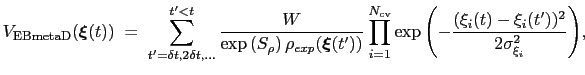
The ensemble-biased metadynamics (EBMetaD) approach [73] is designed to reproduce a target probability distribution along selected collective variables.
Standard metadynamics can be seen as a special case of EBMetaD with a flat distribution as target.
This is achieved by weighing the Gaussian functions used in the metadynamics approach by the inverse of the target probability distribution:
 |
(13.32) |
where
 is the target probability distribution and
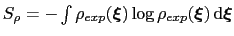 its corresponding differential entropy.
The method is designed so that during the simulation the resulting distribution of the collective variable
converges to
.
A practical application of EBMetaD is to reproduce an ``experimental'' probability distribution, for example the distance distribution between spectroscopic labels inferred from Förster resonance energy transfer (FRET) or double electron-electron resonance (DEER) experiments [73].
its corresponding differential entropy.
The method is designed so that during the simulation the resulting distribution of the collective variable
converges to
.
A practical application of EBMetaD is to reproduce an ``experimental'' probability distribution, for example the distance distribution between spectroscopic labels inferred from Förster resonance energy transfer (FRET) or double electron-electron resonance (DEER) experiments [73].
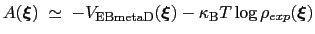
The PMF along
can be estimated from the bias potential and the target ditribution [73]:
 |
(13.33) |
and obtained by enabling writeFreeEnergyFile.
Similarly to eq. 13.32, a more accurate estimate of the free energy can be obtained by averaging (after an equilibration time) multiple time-dependent free energy estimates (see keepFreeEnergyFiles).
The following additional options define the configuration for the ensemble-biased metadynamics approach:
-
ebMeta
Perform ensemble-biased metadynamics
Context: metadynamics
Acceptable values: boolean
Default value: off
Description: If enabled, this flag activates the ensemble-biased metadynamics as
described by Marinelli et al.[73]. The target distribution file,
targetdistfile, is then required. The keywords lowerBoundary, upperBoundary
and width for the respective variables are also needed to set the binning (grid) of the target distribution file.
-
targetDistFile
Target probability distribution file for ensemble-biased metadynamics
Context: metadynamics
Acceptable values: multicolumn text file
Description: This file provides the target probability distribution,
, reported in eq. 13.33. The latter distribution must be a tabulated function provided in a multicolumn text format (see ).
The provided distribution is then normalized.
-
ebMetaEquilSteps
Number of equilibration steps for ensemble-biased metadynamics
Context: metadynamics
Acceptable values: positive integer
Description: The EBMetaD approach may introduce large hills in regions with small values of the target probability distribution (eq. 13.33).
This happens, for example, if the probability distribution sampled by a conventional molecular dynamics simulation is significantly different from the target distribution.
This may lead to instabilities at the beginning of the simulation related to large biasing forces.
In this case, it is useful to introduce an equilibration stage in which the bias potential gradually switches from standard metadynamics (eq. 13.30) to EBmetaD (eq. 13.33) as
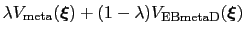 , where
 and step is the current simulation step number.
-
targetDistMinVal
Minimum value of the target distribution in reference to its maximum value
Context: metadynamics
Acceptable values: positive decimal
Description: It is useful to set a minimum value of the target probability distribution to avoid values of the latter that are nearly zero, leading to very large hills.
This parameter sets the minimum value of the target probability distribution that is expressed as a fraction of its maximum value: minimum value =
maximum value X targetDistMinVal. This implies that 0 < targetDistMinVal < 1 and its default value is set to 1/1000000.
To avoid divisions by zero (see eq. 13.33), if targetDistMinVal is set as zero, values of
 equal to zero are replaced by the
smallest positive value read in the same file.
equal to zero are replaced by the
smallest positive value read in the same file.
As with standard metadynamics, multidimensional probability distributions can be targeted using a single metadynamics block using multiple colvars and a multidimensional target distribution file (see ).
Instead, multiple probability distributions on different variables can be targeted separately in the same simulation by introducing multiple metadynamics blocks with the ebMeta option.
Example: EBmetaD configuration for a single variable.
colvar {
name r
distance {
group1 { atomNumbers 991 992 }
group2 { atomNumbers 1762 1763 }
}
upperBoundary 100.0
width 0.1
}
metadynamics {
name ebmeta
colvars r
hillWeight 0.01
hillWidth 3.0
ebMeta on
targetDistFile targetdist1.dat
ebMetaEquilSteps 500000
}
where targetdist1.dat is a text file in ``multicolumn'' format () with the same width as the variable r (0.1 in this case):
| # |
1 |
|
|
|
|
| # |
0.0 |
0.1 |
1000 |
0 |
|
| |
|
|
|
|
|
| |
0.05 |
0.0012 |
|
|
|
| |
0.15 |
0.0014 |
|
|
|
| |
... |
... |
|
|
|
| |
99.95 |
0.0010 |
|
|
|
| |
|
|
|
|
|
Tip: Besides setting a meaninful value for targetDistMinVal, the exploration of unphysically low values of the target distribution (which would lead to very large hills and possibly numerical instabilities) can be also prevented by restricting sampling to a given interval, using e.g. harmonicWalls restraint ().
The following options define the configuration for the ``well-tempered'' metadynamics approach [74]:
Metadynamics calculations can be performed concurrently by multiple replicas that share a common history.
This variant of the method is called multiple-walker metadynamics [75]: the Gaussian hills of all replicas are periodically combined into a single biasing potential, intended to converge to a single PMF.
In the implementation here described [48], replicas communicate through files.
This arrangement allows launching the replicas either (1) as a bundle (i.e. a single job in a cluster's queueing system) or (2) as fully independent runs (i.e. as separate jobs for the queueing system).
One advantage of the use case (1) is that an identical Colvars configuration can be used for all replicas (otherwise, replicaID needs to be manually set to a different string for each replica).
However, the use case (2) is less demanding in terms of high-performance computing resources: a typical scenario would be a computer cluster (including virtual servers from a cloud provider) where not all nodes are connected to each other at high speed, and thus each replica runs on a small group of nodes or a single node.
Whichever way the replicas are started (coupled or not), a shared filesystem is needed so that each replica can read the files created by the others: paths to these files are stored in the shared file replicasRegistry.
This file, and those listed in it, are read every replicaUpdateFrequency steps.
Each time the Colvars state file is written (for example, colvarsRestartFrequency steps), the file named:
outputName.colvars.name.replicaID.state
is written as well; this file contains only the state of the metadynamics bias, which the other replicas will read in turn.
In between the times when this file is modified/replaced, new hills are also temporarily written to the file named:
outputName.colvars.name.replicaID.hills
Both files are only used for communication, and may be deleted after the replica begins writing files with a new outputName.
Example: Multiple-walker metadynamics with file-based communication.
metadynamics {
name mymtd
colvars x
hillWeight 0.001
newHillFrequency 1000
hillWidth 3.0
multipleReplicas on
replicasRegistry /shared-folder/mymtd-replicas.txt
replicaUpdateFrequency 50000 # Best if larger than newHillFrequency
}
The following are the multiple-walkers related options:
-
multipleReplicas
Enable multiple-walker metadynamics
Context: metadynamics
Acceptable values: boolean
Default value: off
Description: This option turns on multiple-walker communication between replicas.
-
replicasRegistry
Multiple replicas database file
Context: metadynamics
Acceptable values: UNIX filename
Description: If multipleReplicas is on, this option sets the path to the replicas' shared database file.
It is best to use an absolute path (especially when running individual replicas in separate folders).
-
replicaUpdateFrequency
How often hills are shared between replicas
Context: metadynamics
Acceptable values: positive integer
Description: If multipleReplicas is on, this option sets the number of steps after which each replica tries to read the other replicas' files.
On a networked file system, it is best to use a number of steps that corresponds to at least a minute of wall time.
-
replicaID
Set the identifier for this replica
Context: metadynamics
Acceptable values: string
Default value: replica index (only if a shared communicator is used)
Description: If multipleReplicas is on, this option sets a unique identifier for this replicas.
When the replicas are launched in a single command (i.e. they share a parallel communicator and are tightly synchronized) this value is optional, and defaults to the replica's numeric index (starting at zero).
However, when the replicas are launched as independent runs this option is required.
-
writePartialFreeEnergyFile
Periodically write the contribution to the
PMF from this replica
Context: metadynamics
Acceptable values: boolean
Default value: off
Description: If multipleReplicas is on, enabling this option produces an additional file outputName.partial.pmf, which can be useful to monitor the contribution of each replica to the total PMF (which is written to the file outputName.pmf).
Note: the name of this file is chosen for consistency and convenience, but its content is not a PMF and it is not expected to converge, even if the total PMF does.
Next: Harmonic restraints
Up: Biasing and analysis methods
Previous: Extended-system Adaptive Biasing Force
Contents
Index
vmd@ks.uiuc.edu