Modeling the quantum system

To describe the input parameters for PHI, first the model of the quantum system has to be specified. The quantum system is described by a total Hamiltonian

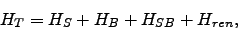$$H_T = H_S + H_B + H_{SB} + H_{ren},$$ (1)

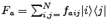
where $H_S$ describes the system of interest, $H_B$ the thermal environment, $H_{SB}$ the system-environment coupling, and $H_{ren}$ is a renormalization term (specified below) dependent on the system-environment coupling. The system Hamiltonian describes states ${\left\vert i \right>}$, $i=1,\cdots,N$ with energies $E_i$ and interaction $V_{ij}$ as

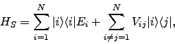$$H_S = \sum_{i=1}^N {\left\vert i \right>}{\left< i \right\ve... ...e j=1}^{N} V_{ij}{\left\vert i \right>}{\left< j \right\vert},$$ (2)

The environment is modeled as an infinite set of harmonic oscillators with

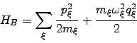$$H_B = \sum_\xi \frac{p_\xi^2}{2m_\xi} + \frac{m_\xi\omega_\xi^2q_\xi^2}{2}$$ (3)

The system-environment coupling is assumed to be linear given by

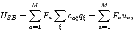$$H_{SB} = \sum_{a=1}^M F_a \sum_\xi c_{a\xi}q_\xi = \sum_{a=1}^M F_a u_a,$$ (4)

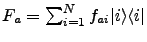
where $F_a = \sum_{i,j=}^N f_{aij} {{\left\vert i \right>}{\left< j \right\vert}}$ specifies the exact form of the coupling. At present only diagonal forms of $F_a$ are implemented in PHI, such that 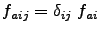${f_{aij} = \delta_{ij}\;f_{ai}}$. In the present implementation only three types of $F_a$ are allowed:

1. diagonal, independent coupling: $M=N$, $F_a={{\left\vert a \right>}{\left< a \right\vert}}$
2. diagonal, independent coupling: $M\ne N$, $F_a = {{\left\vert i_a \right>}{\left< i_a \right\vert}}$ for $i_a \in \left\{1,\cdots,N\right\}$.
3. diagonal, correlated coupling: $M=N$, $F_a = \sum_{i=1}^N f_{ai}{{\left\vert i \right>}{\left< i \right\vert}}$

The coupling introduces a shift in the bath coordinates $q_\xi$ that needs to be countered with the renormalization term

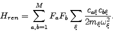$$H_{ren} = \sum_{a,b=1}^M F_{a} F_{b} \sum_\xi \frac{c_{a\xi} c_{b\xi}}{2 m_\xi \omega_\xi^2}.$$ (5)

Note that the renormalization term is NOT added to the system Hamiltonian in PHI - this is left up to the user to include in the Hamiltonian section of the input parameters. PHI implements the HEOM to calculate the system density matrix $\rho(t)$ averaged over environmental fluctuations

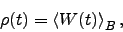$$\rho(t) = \left< W(t) \right>_B,$$ (6)

where $W(t)$ is the density matrix of the complete system + environment. The time evolution of $W(t)$ is formally calculated as

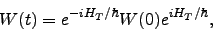$$W(t) = e^{- i H_T / \hbar } W(0) e^{i H_T / \hbar },$$ (7)

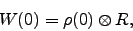
Where $W(0)$ specifies the density matrix of the complete system at $t=0$. Assuming that the environment is in thermal equilibrium and that initially the system and environment are uncorrelated, the initial density matrix is given by

$$W(0) = \rho(0)\otimes R,$$ (8)

where $R = \exp(-\beta H_B)/{\rm tr} _B\left\{{\exp(-\beta H_B)}\right\}$, ${\rm tr} _B$ is the partial trace over bath coordinates and $\beta=1/T$ is the inverse temperature. The system density matrix evolution can be written as

$$\rho(t) = \left< e^{- i H_T / \hbar } \rho(0) e^{i H_T / \hb... ...i H_T / \hbar }\ \rho(0)\otimes R\ e^{i H_T / \hbar } \right\}$$ (9)