


Next: Selecting atoms
Up: Collective Variable-based Calculations (Colvars)
Previous: Enabling and controlling the
Contents
Index
Subsections
Defining collective variables
A collective variable is defined by the keyword colvar followed by its configuration options contained within curly braces:
colvar {
name xi
 other options
function_name {
parameters
atom selection
}
}
There are multiple ways of defining a variable:
- The simplest and most common way way is using one of the precompiled functions (here called ``components''), which are listed in section 9.3.1. For example, using the keyword rmsd (section 9.3.5) defines the variable as the root mean squared deviation (RMSD) of the selected atoms.
- A new variable may also be constructed as a linear or polynomial combination of the components listed in section 9.3.1 (see 9.3.15 for details).
- A user-defined mathematical function of the existing components (see list in section 9.3.1), or of the atomic coordinates directly (see the cartesian keyword in 9.3.8).
The function is defined through the keyword customFunction (see 9.3.16) (see 9.3.16 for details).
- A user-defined Tcl function of the existing components (see list in section 9.3.1), or of the atomic coordinates directly (see the cartesian keyword in 9.3.8).
The function is provided by a separate Tcl script, and referenced through the keyword scriptedFunction (see 9.3.17) (see 9.3.17 for details).
Choosing a component (function) is the only parameter strictly required to define a collective variable.
It is also highly recommended to specify a name for the variable:
- name
Name of this colvar
Context: colvar
Acceptable Values: string
Default Value: ``colvar'' + numeric id
Description: The name is an unique case-sensitive string which allows the
Colvars module to identify this colvar unambiguously; it is also
used in the trajectory file to label to the columns corresponding
to this colvar.
Choosing a function
In this context, the function that computes a colvar is called a component.
A component's choice and definition consists of including in the variable's configuration a keyword indicating the type of function (e.g. rmsd), followed by a definition block specifying the atoms involved (see 9.4) and any additional parameters (cutoffs, ``reference'' values, ...).
At least one component must be chosen to define a variable: if none of the keywords listed below is found, an error is raised.
The following components implement functions with a scalar value (i.e. a real number):
- distance (see 9.3.2): distance between two groups;
- distanceZ (see 9.3.2): projection of a distance vector on an axis;
- distanceXY (see 9.3.2): projection of a distance vector on a plane;
- distanceInv (see 9.3.2): mean distance between two groups of atoms (e.g. NOE-based distance);
- angle (see 9.3.3): angle between three groups;
- dihedral (see 9.3.3): torsional (dihedral) angle between four groups;
- dipoleAngle (see 9.3.3): angle between two groups and dipole of a third group;
- dipoleMagnitude (see 9.3.5): magnitude of the dipole of a group of atoms;
- polarTheta (see 9.3.3): polar angle of a group in spherical coordinates;
- polarPhi (see 9.3.3): azimuthal angle of a group in spherical coordinates;
- coordNum (see 9.3.4): coordination number between two groups;
- selfCoordNum (see 9.3.4): coordination number of atoms within a
group;
- hBond (see 9.3.4): hydrogen bond between two atoms;
- rmsd (see 9.3.5): root mean square deviation (RMSD) from a set of
reference coordinates;
- eigenvector (see 9.3.5): projection of the atomic coordinates on a
vector;
- mapTotal (see 9.3.11): total value of a volumetric map;
- orientationAngle (see 9.3.6): angle of the best-fit rotation from
a set of reference coordinates;
- orientationProj (see 9.3.6): cosine of orientationProj (see 9.3.6);
- spinAngle (see 9.3.6): projection orthogonal to an axis of the best-fit rotation
from a set of reference coordinates;
- tilt (see 9.3.6): projection on an axis of the best-fit rotation
from a set of reference coordinates;
- gyration (see 9.3.5): radius of gyration of a group of atoms;
- inertia (see 9.3.5): moment of inertia of a group of atoms;
- inertiaZ (see 9.3.5): moment of inertia of a group of atoms around a chosen axis;
- alpha (see 9.3.7):
 -helix content of a protein segment.
- dihedralPC (see 9.3.7): projection of protein backbone dihedrals onto a dihedral principal component.
Some components do not return scalar, but vector values:
- distanceVec (see 9.3.2): distance vector between two groups (length: 3);
- distanceDir (see 9.3.2): unit vector parallel to distanceVec (length: 3);
- cartesian (see 9.3.8): vector of atomic Cartesian coordinates (length:
 times the number of Cartesian components requested, X, Y or Z);
- distancePairs (see 9.3.8): vector of mutual distances (length:
 );
);
- orientation (see 9.3.6): best-fit rotation, expressed as a unit quaternion (length: 4).
The types of components used in a colvar (scalar or not) determine the
properties of that colvar, and particularly which biasing or analysis methods
can be applied.
What if ``X'' is not listed? If a function type is not available on this list, it may be possible to define it as a polynomial superposition of existing ones (see 9.3.15), a custom function (see 9.3.16), or a scripted function (see 9.3.17).
In the rest of this section, all available component types are listed, along with their physical units and the ranges of values, if limited.
Such limiting values can be used to define lowerBoundary (see 9.3.18) and upperBoundary (see 9.3.18) in the parent colvar.
For each type of component, the available configurations keywords are listed:
when two components share certain keywords, the second component references to
the documentation of the first one that uses that keyword.
The very few keywords that are available for all types of components are listed in a separate section 9.3.12.
Distances
distance: center-of-mass distance between two groups.
The distance {...} block defines a distance component between the two atom groups, group1 and group2.
List of keywords (see also 9.3.15 for additional options):
- group1
First group of atoms
Context: distance
Acceptable Values: Block group1 {...}
Description: First group of atoms.
-
group2: analogous to group1
- forceNoPBC
Calculate absolute rather than minimum-image distance?
Context: distance
Acceptable Values: boolean
Default Value: no
Description: By default, in calculations with periodic boundary conditions, the
distance component returns the distance according to the
minimum-image convention. If this parameter is set to yes,
PBC will be ignored and the distance between the coordinates as maintained
internally will be used. This is only useful in a limited number of
special cases, e.g. to describe the distance between remote points
of a single macromolecule, which cannot be split across periodic cell
boundaries, and for which the minimum-image distance might give the
wrong result because of a relatively small periodic cell.
- oneSiteTotalForce
Measure total force on group 1 only?
Context: angle, dipoleAngle, dihedral
Acceptable Values: boolean
Default Value: no
Description: If this is set to yes, the total force is measured along
a vector field (see equation (61) in
section 9.5.2) that only involves atoms of
group1. This option is only useful for ABF, or custom
biases that compute total forces. See
section 9.5.2 for details.
The value returned is a positive number (in Å), ranging from 0
to the largest possible interatomic distance within the chosen
boundary conditions (with PBCs, the minimum image convention is used
unless the forceNoPBC option is set).
distanceZ: projection of a distance vector on an axis.
The distanceZ {...} block defines a distance projection
component, which can be seen as measuring the distance between two
groups projected onto an axis, or the position of a group along such
an axis. The axis can be defined using either one reference group and
a constant vector, or dynamically based on two reference groups.
One of the groups can be set to a dummy atom to allow the use of an absolute Cartesian coordinate.
List of keywords (see also 9.3.15 for additional options):
This component returns a number (in Å) whose range is determined
by the chosen boundary conditions. For instance, if the  axis is
used in a simulation with periodic boundaries, the returned value ranges
between
axis is
used in a simulation with periodic boundaries, the returned value ranges
between  and
and  , where
  is the box length
along
(this behavior is disabled if forceNoPBC is set).
is the box length
along
(this behavior is disabled if forceNoPBC is set).
distanceXY: modulus of the projection of a distance vector on a plane.
The distanceXY {...} block defines a distance projected on
a plane, and accepts the same keywords as the component distanceZ, i.e.
main, ref, either ref2 or axis,
and oneSiteTotalForce. It returns the norm of the
projection of the distance vector between main and
ref onto the plane orthogonal to the axis. The axis is
defined using the axis parameter or as the vector joining
ref and ref2 (see distanceZ above).
List of keywords (see also 9.3.15 for additional options):
-
main: see definition of main in sec. 9.3.2 (distanceZ component)
-
ref: see definition of ref in sec. 9.3.2 (distanceZ component)
-
ref2: see definition of ref2 in sec. 9.3.2 (distanceZ component)
-
axis: see definition of axis in sec. 9.3.2 (distanceZ component)
-
forceNoPBC: see definition of forceNoPBC in sec. 9.3.2 (distance component)
-
oneSiteTotalForce: see definition of oneSiteTotalForce in sec. 9.3.2 (distance component)
distanceVec: distance vector between two groups.
The distanceVec {...} block defines
a distance vector component, which accepts the same keywords as
the component distance: group1, group2, and
forceNoPBC. Its value is the 3-vector joining the centers
of mass of group1 and group2.
List of keywords (see also 9.3.15 for additional options):
-
group1: see definition of group1 in sec. 9.3.2 (distance component)
-
group2: analogous to group1
-
forceNoPBC: see definition of forceNoPBC in sec. 9.3.2 (distance component)
-
oneSiteTotalForce: see definition of oneSiteTotalForce in sec. 9.3.2 (distance component)
distanceDir: distance unit vector between two groups.
The distanceDir {...} block defines
a distance unit vector component, which accepts the same keywords as
the component distance: group1, group2, and
forceNoPBC. It returns a
3-dimensional unit vector
 , with
 .
.
List of keywords (see also 9.3.15 for additional options):
-
group1: see definition of group1 in sec. 9.3.2 (distance component)
-
group2: analogous to group1
-
forceNoPBC: see definition of forceNoPBC in sec. 9.3.2 (distance component)
-
oneSiteTotalForce: see definition of oneSiteTotalForce in sec. 9.3.2 (distance component)
distanceInv: mean distance between two groups of atoms.
The distanceInv {...} block defines a generalized mean distance between two groups of atoms 1 and 2, weighted with exponent  :
:
![$\displaystyle d_{\mathrm{1,2}}^{[n]} \; = \; \left(\frac{1}{N_{\mathrm{1}}N_{\m...
...}\sum_{i,j} \left(\frac{1}{\Vert\mathbf{d}^{ij}\Vert}\right)^{n} \right)^{-1/n}$](img287.png) |
(36) |
where
 is the distance between atoms
  and
and  in groups 1 and 2 respectively, and
  is an even integer.
List of keywords (see also 9.3.15 for additional options):
-
group1: see definition of group1 in sec. 9.3.2 (distance component)
-
group2: analogous to group1
-
oneSiteTotalForce: see definition of oneSiteTotalForce in sec. 9.3.2 (distance component)
- exponent
Exponent
in equation 36
Context: distanceInv
Acceptable Values: positive even integer
Default Value: 6
Description: Defines the exponent to which the individual distances are elevated before averaging. The default value of 6 is useful for example to applying restraints based on NOE-measured distances.
This component returns a number in Å, ranging from 0
to the largest possible distance within the chosen boundary conditions.
Angles
angle: angle between three groups.
The angle {...} block defines an angle, and contains the
three blocks group1, group2 and group3, defining
the three groups. It returns an angle (in degrees) within the
interval ![$ [0:180]$](img289.png) .
.
List of keywords (see also 9.3.15 for additional options):
-
group1: see definition of group1 in sec. 9.3.2 (distance component)
-
group2: analogous to group1
-
group3: analogous to group1
-
forceNoPBC: see definition of forceNoPBC in sec. 9.3.2 (distance component)
-
oneSiteTotalForce: see definition of oneSiteTotalForce in sec. 9.3.2 (distance component)
dipoleAngle: angle between two groups and dipole of a third group.
The dipoleAngle {...} block defines an angle, and contains the
three blocks group1, group2 and group3, defining
the three groups, being group1 the group where dipole is calculated.
It returns an angle (in degrees) within the interval
.
List of keywords (see also 9.3.15 for additional options):
-
group1: see definition of group1 in sec. 9.3.2 (distance component)
-
group2: analogous to group1
-
group3: analogous to group1
-
forceNoPBC: see definition of forceNoPBC in sec. 9.3.2 (distance component)
-
oneSiteTotalForce: see definition of oneSiteTotalForce in sec. 9.3.2 (distance component)
dihedral: torsional angle between four groups.
The dihedral {...} block defines a torsional angle, and
contains the blocks group1, group2, group3
and group4, defining the four groups. It returns an angle
(in degrees) within the interval
![$ [-180:180]$](img290.png) . The Colvars module
calculates all the distances between two angles taking into account
periodicity. For instance, reference values for restraints or range
boundaries can be defined by using any real number of choice.
. The Colvars module
calculates all the distances between two angles taking into account
periodicity. For instance, reference values for restraints or range
boundaries can be defined by using any real number of choice.
List of keywords (see also 9.3.15 for additional options):
-
group1: see definition of group1 in sec. 9.3.2 (distance component)
-
group2: analogous to group1
-
group3: analogous to group1
-
group4: analogous to group1
-
forceNoPBC: see definition of forceNoPBC in sec. 9.3.2 (distance component)
-
oneSiteTotalForce: see definition of oneSiteTotalForce in sec. 9.3.2 (distance component)
polarTheta: polar angle in spherical coordinates.
The polarTheta {...} block defines the polar angle in
spherical coordinates, for the center of mass of a group of atoms
described by the block atoms. It returns an angle
(in degrees) within the interval
.
To obtain spherical coordinates in a frame of reference tied to
another group of atoms, use the fittingGroup (9.4.2) option
within the atoms block.
An example is provided in file examples/11_polar_angles.in of the Colvars public repository.
List of keywords (see also 9.3.15 for additional options):
- atoms
Atom group
Context: polarPhi
Acceptable Values: atoms {...} block
Description: Defines the group of atoms for the COM of which the angle should be calculated.
polarPhi: azimuthal angle in spherical coordinates.
The polarPhi {...} block defines the azimuthal angle in
spherical coordinates, for the center of mass of a group of atoms
described by the block atoms. It returns an angle
(in degrees) within the interval
. The Colvars module
calculates all the distances between two angles taking into account
periodicity. For instance, reference values for restraints or range
boundaries can be defined by using any real number of choice.
To obtain spherical coordinates in a frame of reference tied to
another group of atoms, use the fittingGroup (9.4.2) option
within the atoms block.
An example is provided in file examples/11_polar_angles.in of the Colvars public repository.
List of keywords (see also 9.3.15 for additional options):
- atoms
Atom group
Context: polarPhi
Acceptable Values: atoms {...} block
Description: Defines the group of atoms for the COM of which the angle should be calculated.
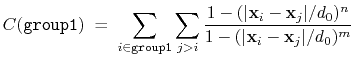
Contacts
coordNum: coordination number between two groups.
The coordNum {...} block defines
a coordination number (or number of contacts), which calculates the
function
 , where
  is the
``cutoff'' distance, and
and
is the
``cutoff'' distance, and
and  are exponents that can control
its long range behavior and stiffness [49]. This
function is summed over all pairs of atoms in group1 and
group2:
are exponents that can control
its long range behavior and stiffness [49]. This
function is summed over all pairs of atoms in group1 and
group2:
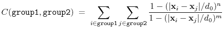 |
(37) |
List of keywords (see also 9.3.15 for additional options):
-
group1: see definition of group1 in sec. 9.3.2 (distance component)
-
group2: analogous to group1
- cutoff
``Interaction'' distance (Å)
Context: coordNum
Acceptable Values: positive decimal
Default Value: 4.0
Description: This number defines the switching distance to define an
interatomic contact: for  , the switching function
is close to 1, at
, the switching function
is close to 1, at  it
has a value of
it
has a value of  (
( with the default
and
), and at
with the default
and
), and at
 it goes to zero approximately like
  . Hence,
for a proper behavior,
must be larger than
.
. Hence,
for a proper behavior,
must be larger than
.
- cutoff3
Reference distance vector (Å)
Context: coordNum
Acceptable Values: ``(x, y, z)'' triplet of positive decimals
Default Value: (4.0, 4.0, 4.0)
Description: The three components of this vector define three different cutoffs
 for each direction. This option is mutually exclusive with
cutoff.
for each direction. This option is mutually exclusive with
cutoff.
- expNumer
Numerator exponent
Context: coordNum
Acceptable Values: positive even integer
Default Value: 6
Description: This number defines the
exponent for the switching function.
- expDenom
Denominator exponent
Context: coordNum
Acceptable Values: positive even integer
Default Value: 12
Description: This number defines the
exponent for the switching function.
- group2CenterOnly
Use only group2's center of
mass
Context: coordNum
Acceptable Values: boolean
Default Value: off
Description: If this option is on, only contacts between each atoms in group1 and the center of mass of group2 are calculated (by default, the sum extends over all pairs of atoms in group1 and group2).
If group2 is a dummyAtom, this option is set to yes by default.
- tolerance
Pairlist control
Context: coordNum
Acceptable Values: decimal
Default Value: 0.0
Description: This controls the pairlist feature, dictating the minimum value for each summation element in Eq. 37 such that the pair that contributed the summation element is included in subsequent simulation timesteps until the next pairlist recalculation. For most applications, this value should be small (eg. 0.001) to avoid missing important contributions to the overall sum. Higher values will improve performance by reducing the number of pairs that contribute to the sum. Values above 1 will exclude all possible pair interactions. Similarly, values below 0 will never exclude a pair from consideration. To ensure continuous forces, Eq. 37 is further modified by subtracting the tolerance and then rescaling so that each pair covers the range
![$ \left[0, 1\right]$](img302.png) .
.
- pairListFrequency
Pairlist regeneration frequency
Context: coordNum
Acceptable Values: positive integer
Default Value: 100
Description: This controls the pairlist feature, dictating how many steps are taken between regenerating pairlists if the tolerance is greater than 0.
This component returns a dimensionless number, which ranges from
approximately 0 (all interatomic distances are much larger than the
cutoff) to
 (all distances
are less than the cutoff), or
(all distances
are less than the cutoff), or
 if
group2CenterOnly is used. For performance reasons, at least
one of group1 and group2 should be of limited size or group2CenterOnly should be used: the cost of the loop over all pairs grows as
.
Setting
if
group2CenterOnly is used. For performance reasons, at least
one of group1 and group2 should be of limited size or group2CenterOnly should be used: the cost of the loop over all pairs grows as
.
Setting
 ameliorates this to some degree, although every pair is still checked to regenerate the pairlist.
selfCoordNum: coordination number between atoms within a group.
The selfCoordNum {...} block defines
a coordination number similarly to the component coordNum,
but the function is summed over atom pairs within group1:
 |
(38) |
The keywords accepted by selfCoordNum are a subset of
those accepted by coordNum, namely group1
(here defining all of the atoms to be considered),
cutoff, expNumer, and expDenom.
List of keywords (see also 9.3.15 for additional options):
-
group1: see definition of group1 in sec. 9.3.4 (coordNum component)
-
cutoff: see definition of cutoff in sec. 9.3.4 (coordNum component)
-
cutoff3: see definition of cutoff3 in sec. 9.3.4 (coordNum component)
-
expNumer: see definition of expNumer in sec. 9.3.4 (coordNum component)
-
expDenom: see definition of expDenom in sec. 9.3.4 (coordNum component)
-
tolerance: see definition of tolerance in sec. 9.3.4 (coordNum component)
-
pairListFrequency: see definition of pairListFrequency in sec. 9.3.4 (coordNum component)
This component returns a dimensionless number, which ranges from
approximately 0 (all interatomic distances much larger than the
cutoff) to
 (all
distances within the cutoff). For performance reasons,
group1 should be of limited size, because the cost of the
loop over all pairs grows as
(all
distances within the cutoff). For performance reasons,
group1 should be of limited size, because the cost of the
loop over all pairs grows as
 .
.
hBond: hydrogen bond between two atoms.
The hBond {...} block defines a hydrogen
bond, implemented as a coordination number (eq. 37)
between the donor and the acceptor atoms. Therefore, it accepts the
same options cutoff (with a different default value of
3.3 Å), expNumer (with a default value of 6) and
expDenom (with a default value of 8). Unlike
coordNum, it requires two atom numbers, acceptor and
donor, to be defined. It returns an adimensional number,
with values between 0 (acceptor and donor far outside the cutoff
distance) and 1 (acceptor and donor much closer than the cutoff).
List of keywords (see also 9.3.15 for additional options):
- acceptor
Number of the acceptor atom
Context: hBond
Acceptable Values: positive integer
Description: Number that uses the same convention as atomNumbers.
-
donor: analogous to acceptor
-
cutoff: see definition of cutoff in sec. 9.3.4 (coordNum component)
Note: default value is 3.3 Å.
-
expNumer: see definition of expNumer in sec. 9.3.4 (coordNum component)
Note: default value is 6.
-
expDenom: see definition of expDenom in sec. 9.3.4 (coordNum component)
Note: default value is 8.
Collective metrics
rmsd: root mean square displacement (RMSD) from reference positions.
The block rmsd {...} defines the root mean square replacement
(RMSD) of a group of atoms with respect to a reference structure. For
each set of coordinates
 , the colvar component rmsd calculates the
optimal rotation
, the colvar component rmsd calculates the
optimal rotation
 that best superimposes the coordinates
 onto a
set of reference coordinates
onto a
set of reference coordinates
 .
Both the current and the reference coordinates are centered on their
centers of geometry,
.
Both the current and the reference coordinates are centered on their
centers of geometry,
 and
and
 . The root mean square
displacement is then defined as:
. The root mean square
displacement is then defined as:
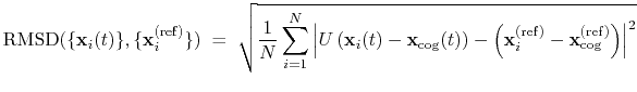 |
(39) |
The optimal rotation
is calculated within the formalism developed in
reference [26], which guarantees a continuous
dependence of
with respect to
.
List of keywords (see also 9.3.15 for additional options):
- atoms
Atom group
Context: rmsd
Acceptable Values: atoms {...} block
Description: Defines the group of atoms of which the RMSD should be calculated.
Optimal fit options (such as refPositions and
rotateReference) should typically NOT be set within this
block. Exceptions to this rule are the special cases discussed in
the Advanced usage paragraph below.
- refPositions
Reference coordinates
Context: rmsd
Acceptable Values: space-separated list of (x, y, z) triplets
Description: This option (mutually exclusive with refPositionsFile) sets the reference coordinates for RMSD calculation, and uses these to compute the roto-translational fit.
It is functionally equivalent to the option refPositions (see 9.4.2) in the atom group definition, which also supports more advanced fitting options.
- refPositionsFile
Reference coordinates file
Context: rmsd
Acceptable Values: UNIX filename
Description: This option (mutually exclusive with refPositions) sets the reference coordinates for RMSD calculation, and uses these to compute the roto-translational fit.
It is functionally equivalent to the option refPositionsFile (see 9.4.2) in the atom group definition, which also supports more advanced fitting options.
- refPositionsCol
PDB column containing atom flags
Context: rmsd
Acceptable Values: O, B, X, Y, or Z
Description: If refPositionsFile is a PDB file that contains all the atoms in the topology, this option may be provided to set which PDB field is used to flag the reference coordinates for atoms.
- refPositionsColValue
Atom selection flag in the PDB column
Context: rmsd
Acceptable Values: positive decimal
Description: If defined, this value identifies in the PDB column
refPositionsCol of the file refPositionsFile
which atom positions are to be read. Otherwise, all positions
with a non-zero value are read.
- atomPermutation
Alternate ordering of atoms for RMSD computation
Context: rmsd
Acceptable Values: List of atom numbers
Description: If defined, this parameter defines a re-ordering (permutation) of the 1-based atom numbers that
can be used to compute the RMSD, typically due to molecular symmetry.
This parameter can be specified multiple times, each one defining a new permutation:
the returned RMSD value is the minimum over the set of permutations.
For example, if the atoms making up the group are 6, 7, 8, 9, and atoms 7, 8, and 9
are invariant by circular permutation (as the hydrogens in a CH3 group), a
symmetry-adapted RMSD would be obtained by adding:
atomPermutation 6 8 9 7
atomPermutation 6 9 7 8
Note that this does not affect the least-squares roto-translational fit,
which is done using the topology ordering of atoms, and the reference
positions in the order provided.
Therefore, this feature is mostly useful when using custom fitting parameters within the
atom group, such as fittingGroup (see 9.4.2), or when fitting
is disabled altogether.
This component returns a positive real number (in Å).
Advanced usage of the rmsd component.
In the standard usage as described above, the rmsd component
calculates a minimum RMSD, that is, current coordinates are optimally
fitted onto the same reference coordinates that are used to
compute the RMSD value. The fit itself is handled by the atom group
object, whose parameters are automatically set by the rmsd
component.
For very specific applications, however, it may be
useful to control the fitting process separately from the definition
of the reference coordinates, to evaluate various types of
non-minimal RMSD values. This can be achieved by setting the
related options (refPositions, etc.) explicitly in the
atom group block. This allows for the following non-standard cases:
- applying the optimal translation, but no rotation
(rotateReference off), to bias or restrain the shape and
orientation, but not the position of the atom group;
- applying the optimal rotation, but no translation
(centerReference off), to bias or restrain the shape and
position, but not the orientation of the atom group;
- disabling the application of optimal roto-translations, which
lets the RMSD component describe the deviation of atoms
from fixed positions in the laboratory frame: this allows for custom
positional restraints within the Colvars module;
- fitting the atomic positions to different reference coordinates
than those used in the RMSD calculation itself
(by specifying refPositions (see 9.4.2) or refPositionsFile (see 9.4.2)
within the atom group as well as within the rmsd block);
- applying the optimal rotation and/or translation from a separate
atom group, defined through fittingGroup:
the RMSD then reflects the deviation from reference coordinates in a separate, moving
reference frame (see example in the section on fittingGroup (see 9.4.2)).
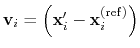
eigenvector: projection of the atomic coordinates on a vector.
The block eigenvector {...} defines the projection of the coordinates
of a group of atoms (or more precisely, their deviations from the
reference coordinates) onto a vector in
 , where
is the
number of atoms in the group. The computed quantity is the
total projection:
, where
is the
number of atoms in the group. The computed quantity is the
total projection:
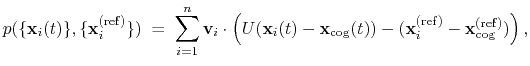 |
(40) |
where, as in the rmsd component,  is the optimal rotation
matrix,
and
are the centers of
geometry of the current and reference positions respectively, and
is the optimal rotation
matrix,
and
are the centers of
geometry of the current and reference positions respectively, and
 are the components of the vector for each atom.
Example choices for
are the components of the vector for each atom.
Example choices for
 are an eigenvector
of the covariance matrix (essential mode), or a normal
mode of the system. It is assumed that
are an eigenvector
of the covariance matrix (essential mode), or a normal
mode of the system. It is assumed that
 :
otherwise, the Colvars module centers the
automatically when reading them from the configuration.
:
otherwise, the Colvars module centers the
automatically when reading them from the configuration.
List of keywords (see also 9.3.15 for additional options):
-
atoms: see definition of atoms in sec. 9.3.5 (rmsd component)
-
refPositions: see definition of refPositions in sec. 9.3.5 (rmsd component)
-
refPositionsFile: see definition of refPositionsFile in sec. 9.3.5 (rmsd component)
-
refPositionsCol: see definition of refPositionsCol in sec. 9.3.5 (rmsd component)
-
refPositionsColValue: see definition of refPositionsColValue in sec. 9.3.5 (rmsd component)
- vector
Vector components
Context: eigenvector
Acceptable Values: space-separated list of (x, y, z) triplets
Description: This option (mutually exclusive with vectorFile) sets the values of the vector components.
- vectorFile
file containing vector components
Context: eigenvector
Acceptable Values: UNIX filename
Description: This option (mutually exclusive with vector) sets the name of a coordinate file containing the vector components; the file is read according to the same format used for refPositionsFile.
For a PDB file specifically, the components are read from the X, Y and Z fields.
Note: The PDB file has limited precision and fixed-point numbers: in some cases, the vector components may not be accurately represented; a XYZ file should be used instead, containing floating-point numbers.
- vectorCol
PDB column used to flag participating atoms
Context: eigenvector
Acceptable Values: O or B
Description: Analogous to atomsCol.
- vectorColValue
Value used to flag participating atoms in the PDB file
Context: eigenvector
Acceptable Values: positive decimal
Description: Analogous to atomsColValue.
- differenceVector
The
 -dimensional vector is the difference between vector and refPositions
Context: eigenvector
Acceptable Values: boolean
Default Value: off
Description: If this option is on, the numbers provided by vector or vectorFile are interpreted as another set of positions,
 : the vector
is then defined as
: the vector
is then defined as
 .
This allows to conveniently define a colvar
.
This allows to conveniently define a colvar  as a projection on the linear transformation between two sets of positions, ``A'' and ``B''.
For convenience, the vector is also normalized so that
as a projection on the linear transformation between two sets of positions, ``A'' and ``B''.
For convenience, the vector is also normalized so that  when the atoms are at the set of positions ``A'' and
  at the set of positions ``B''.
This component returns a number (in Å), whose value ranges between
the smallest and largest absolute positions in the unit cell during
the simulations (see also distanceZ). Due to the
normalization in eq. 40, this range does not
depend on the number of atoms involved.
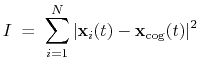
gyration: radius of gyration of a group of atoms.
The block gyration {...} defines the
parameters for calculating the radius of gyration of a group of atomic
positions
with respect to their center of geometry,
:
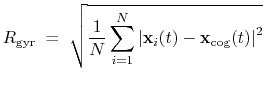 |
(41) |
This component must contain one atoms {...} block to
define the atom group, and returns a positive number, expressed in
Å.
List of keywords (see also 9.3.15 for additional options):
-
atoms: see definition of atoms in sec. 9.3.5 (rmsd component)
inertia: total moment of inertia of a group of atoms.
The block inertia {...} defines the
parameters for calculating the total moment of inertia of a group of atomic
positions
with respect to their center of geometry,
:
 |
(42) |
Note that all atomic masses are set to 1 for simplicity.
This component must contain one atoms {...} block to
define the atom group, and returns a positive number, expressed in
Å .
.
List of keywords (see also 9.3.15 for additional options):
-
atoms: see definition of atoms in sec. 9.3.5 (rmsd component)
dipoleMagnitude: dipole magnitude of a group of atoms.
The dipoleMagnitude {...} block defines the dipole magnitude of a group of atoms (norm of the dipole moment's vector), being atoms the group where dipole magnitude is calculated.
It returns the magnitude in elementary charge  times Å.
List of keywords (see also 9.3.15 for additional options):
-
atoms: see definition of atoms in sec. 9.3.5 (rmsd component)
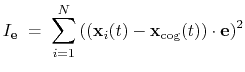
inertiaZ: total moment of inertia of a group of atoms around a chosen axis.
The block inertiaZ {...} defines the
parameters for calculating the component along the axis
 of the moment of inertia of a group of atomic
positions
with respect to their center of geometry,
:
of the moment of inertia of a group of atomic
positions
with respect to their center of geometry,
:
 |
(43) |
Note that all atomic masses are set to 1 for simplicity.
This component must contain one atoms {...} block to
define the atom group, and returns a positive number, expressed in
Å
.
List of keywords (see also 9.3.15 for additional options):
-
atoms: see definition of atoms in sec. 9.3.5 (rmsd component)
- axis
Projection axis (Å)
Context: inertiaZ
Acceptable Values: (x, y, z) triplet
Default Value: (0.0, 0.0, 1.0)
Description: The three components of this vector define (when normalized) the
projection axis
.
Rotations
orientation: orientation from reference coordinates.
The block orientation {...} returns the
same optimal rotation used in the rmsd component to
superimpose the coordinates
onto a set of
reference coordinates
. Such
component returns a four dimensional vector
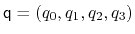 , with
 ; this quaternion
expresses the optimal rotation
; this quaternion
expresses the optimal rotation
 according to the formalism in
reference [26]. The quaternion
according to the formalism in
reference [26]. The quaternion
 can also be written as
 , where
  is the angle and
 the normalized axis of rotation; for example, a rotation
of 90
the normalized axis of rotation; for example, a rotation
of 90 around the
axis is expressed as
``(0.707, 0.0, 0.0, 0.707)''. The script
quaternion2rmatrix.tcl provides Tcl functions for converting
to and from a
around the
axis is expressed as
``(0.707, 0.0, 0.0, 0.707)''. The script
quaternion2rmatrix.tcl provides Tcl functions for converting
to and from a
 rotation matrix in a format suitable for
usage in VMD.
rotation matrix in a format suitable for
usage in VMD.
As for the component rmsd, the available options are atoms, refPositionsFile, refPositionsCol and refPositionsColValue, and refPositions.
Note: refPositionsand refPositionsFile define the set of positions from which the optimal rotation is calculated, but this rotation is not applied to the coordinates of the atoms involved: it is used instead to define the variable itself.
List of keywords (see also 9.3.15 for additional options):
-
atoms: see definition of atoms in sec. 9.3.5 (rmsd component)
-
refPositions: see definition of refPositions in sec. 9.3.5 (rmsd component)
-
refPositionsFile: see definition of refPositionsFile in sec. 9.3.5 (rmsd component)
-
refPositionsCol: see definition of refPositionsCol in sec. 9.3.5 (rmsd component)
-
refPositionsColValue: see definition of refPositionsColValue in sec. 9.3.5 (rmsd component)
- closestToQuaternion
Reference rotation
Context: orientation
Acceptable Values: ``(q0, q1, q2, q3)'' quadruplet
Default Value: (1.0, 0.0, 0.0, 0.0) (``null'' rotation)
Description: Between the two equivalent quaternions
and
 , the closer to (1.0, 0.0, 0.0,
0.0) is chosen. This simplifies the visualization of the
colvar trajectory when sampled values are a smaller subset of all
possible rotations. Note: this only affects the
output, never the dynamics.
, the closer to (1.0, 0.0, 0.0,
0.0) is chosen. This simplifies the visualization of the
colvar trajectory when sampled values are a smaller subset of all
possible rotations. Note: this only affects the
output, never the dynamics.
Tip: stopping the rotation of a protein. To stop the
rotation of an elongated macromolecule in solution (and use an
anisotropic box to save water molecules), it is possible to define a
colvar with an orientation component, and restrain it through
the harmonic bias around the identity rotation, (1.0,
0.0, 0.0, 0.0). Only the overall orientation of the macromolecule
is affected, and not its internal degrees of freedom. The user
should also take care that the macromolecule is composed by a single
chain, or disable wrapAll otherwise.
orientationAngle: angle of rotation from reference coordinates.
The block orientationAngle {...} accepts the same base options as
the component orientation: atoms, refPositions, refPositionsFile, refPositionsCol and refPositionsColValue.
The returned value is the angle of rotation
between the current and the reference positions.
This angle is expressed in degrees within the range [0
:180
].
List of keywords (see also 9.3.15 for additional options):
-
atoms: see definition of atoms in sec. 9.3.5 (rmsd component)
-
refPositions: see definition of refPositions in sec. 9.3.5 (rmsd component)
-
refPositionsFile: see definition of refPositionsFile in sec. 9.3.5 (rmsd component)
-
refPositionsCol: see definition of refPositionsCol in sec. 9.3.5 (rmsd component)
-
refPositionsColValue: see definition of refPositionsColValue in sec. 9.3.5 (rmsd component)
orientationProj: cosine of the angle of rotation from reference coordinates.
The block orientationProj {...} accepts the same base options as
the component orientation: atoms, refPositions, refPositionsFile, refPositionsCol and refPositionsColValue.
The returned value is the cosine of the angle of rotation
between the current and the reference positions.
The range of values is [-1:1].
List of keywords (see also 9.3.15 for additional options):
-
atoms: see definition of atoms in sec. 9.3.5 (rmsd component)
-
refPositions: see definition of refPositions in sec. 9.3.5 (rmsd component)
-
refPositionsFile: see definition of refPositionsFile in sec. 9.3.5 (rmsd component)
-
refPositionsCol: see definition of refPositionsCol in sec. 9.3.5 (rmsd component)
-
refPositionsColValue: see definition of refPositionsColValue in sec. 9.3.5 (rmsd component)
spinAngle: angle of rotation around a given axis.
The complete rotation described by orientation can optionally be decomposed into two sub-rotations: one is a ``spin'' rotation around e, and the other a ``tilt'' rotation around an axis orthogonal to e.
The component spinAngle measures the angle of the ``spin'' sub-rotation around e.
List of keywords (see also 9.3.15 for additional options):
-
atoms: see definition of atoms in sec. 9.3.5 (rmsd component)
-
refPositions: see definition of refPositions in sec. 9.3.5 (rmsd component)
-
refPositionsFile: see definition of refPositionsFile in sec. 9.3.5 (rmsd component)
-
refPositionsCol: see definition of refPositionsCol in sec. 9.3.5 (rmsd component)
-
refPositionsColValue: see definition of refPositionsColValue in sec. 9.3.5 (rmsd component)
- axis
Special rotation axis (Å)
Context: tilt
Acceptable Values: (x, y, z) triplet
Default Value: (0.0, 0.0, 1.0)
Description: The three components of this vector define (when normalized) the special rotation axis used to calculate the tilt and spinAngle components.
The component spinAngle returns an angle (in degrees) within the periodic interval
.
Note: the value of spinAngle is a continuous function almost everywhere, with the exception of configurations with the corresponding ``tilt'' angle equal to 180 (i.e. the tilt component is equal to
  ): in those cases, spinAngle is undefined. If such configurations are expected, consider defining a tilt colvar using the same axis e, and restraining it with a lower wall away from
.
): in those cases, spinAngle is undefined. If such configurations are expected, consider defining a tilt colvar using the same axis e, and restraining it with a lower wall away from
.
tilt: cosine of the rotation orthogonal to a given axis.
The component tilt measures the cosine of the angle of the ``tilt'' sub-rotation, which combined with the ``spin'' sub-rotation provides the complete rotation of a group of atoms.
The cosine of the tilt angle rather than the tilt angle itself is implemented, because the latter is unevenly distributed even for an isotropic system: consider as an analogy the angle
in the spherical coordinate system.
The component tilt relies on the same options as spinAngle, including the definition of the axis e.
The values of tilt are real numbers in the interval ![$ [-1:1]$](img344.png) : the value
: the value  represents an orientation fully parallel to e (tilt angle = 0
), and the value
represents an anti-parallel orientation.
represents an orientation fully parallel to e (tilt angle = 0
), and the value
represents an anti-parallel orientation.
List of keywords (see also 9.3.15 for additional options):
-
atoms: see definition of atoms in sec. 9.3.5 (rmsd component)
-
refPositions: see definition of refPositions in sec. 9.3.5 (rmsd component)
-
refPositionsFile: see definition of refPositionsFile in sec. 9.3.5 (rmsd component)
-
refPositionsCol: see definition of refPositionsCol in sec. 9.3.5 (rmsd component)
-
refPositionsColValue: see definition of refPositionsColValue in sec. 9.3.5 (rmsd component)
-
axis: see definition of axis in sec. 9.3.6 (spinAngle component)
Protein structure descriptors
alpha:
-helix content of a protein segment.
The block alpha {...} defines the
parameters to calculate the helical content of a segment of protein
residues. The
-helical content across the  residues
 to
to  is calculated by the formula:
 |
|
|
(44) |
 |
|
|
|
where the score function for the
 angle is defined as:
 |
(45) |
and the score function for the
 hydrogen bond is defined through a hBond
colvar component on the same atoms.
hydrogen bond is defined through a hBond
colvar component on the same atoms.
List of keywords (see also 9.3.15 for additional options):
This component returns positive values, always comprised between 0
(lowest
-helical score) and 1 (highest
-helical
score).
dihedralPC: protein dihedral principal component
The block dihedralPC {...} defines the
parameters to calculate the projection of backbone dihedral angles within
a protein segment onto a dihedral principal component, following
the formalism of dihedral principal component analysis (dPCA) proposed by
Mu et al.[79] and documented in detail by Altis et
al.[2].
Given a peptide or protein segment of
residues, each with Ramachandran
angles  and
and  , dPCA rests on a variance/covariance analysis
of the
, dPCA rests on a variance/covariance analysis
of the  variables
 . Note that angles
  and
and  have little impact on chain conformation, and are therefore discarded,
following the implementation of dPCA in the analysis software Carma.[39]
have little impact on chain conformation, and are therefore discarded,
following the implementation of dPCA in the analysis software Carma.[39]
For a given principal component (eigenvector) of coefficients
 ,
the projection of the current backbone conformation is:
,
the projection of the current backbone conformation is:
 |
(46) |
dihedralPC expects the same parameters as the alpha
component for defining the relevant residues (residueRange
and psfSegID) in addition to the following:
List of keywords (see also 9.3.15 for additional options):
-
residueRange: see definition of residueRange in sec. 9.3.7 (alpha component)
-
psfSegID: see definition of psfSegID in sec. 9.3.7 (alpha component)
- vectorFile
File containing dihedral PCA eigenvector(s)
Context: dihedralPC
Acceptable Values: file name
Description: A text file containing the coefficients of dihedral PCA eigenvectors on the
cosine and sine coordinates. The vectors should be arranged in columns,
as in the files output by Carma.[39]
- vectorNumber
File containing dihedralPCA eigenvector(s)
Context: dihedralPC
Acceptable Values: positive integer
Description: Number of the eigenvector to be used for this component.
Raw data: building blocks for custom functions
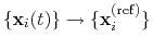
cartesian: vector of atomic Cartesian coordinates.
The cartesian {...} block defines a component returning a flat vector containing
the Cartesian coordinates of all participating atoms, in the order
 .
.
List of keywords (see also 9.3.15 for additional options):
- atoms
Group of atoms
Context: cartesian
Acceptable Values: Block atoms {...}
Description: Defines the atoms whose coordinates make up the value of the component.
If rotateReference or centerReference are defined, coordinates
are evaluated within the moving frame of reference.
distancePairs: set of pairwise distances between two groups.
The distancePairs {...} block defines a
-dimensional variable that includes all mutual distances between the atoms of two groups.
This can be useful, for example, to develop a new variable defined over two groups, by using the scriptedFunction feature.
List of keywords (see also 9.3.15 for additional options):
-
group1: see definition of group1 in sec. 9.3.2 (distance component)
-
group2: analogous to group1
-
forceNoPBC: see definition of forceNoPBC in sec. 9.3.2 (distance component)
This component returns a
-dimensional vector of numbers, each ranging from 0
to the largest possible distance within the chosen boundary conditions.
Geometric path collective variables
The geometric path collective variables define the progress along a path,  , and the distance from the path,
. These CVs are proposed by Leines and Ensing[63] , which differ from that[12] proposed by Branduardi et al., and utilize a set of geometric algorithms. The path is defined as a series of frames in the atomic Cartesian coordinate space or the CV space.
and
are computed as
, and the distance from the path,
. These CVs are proposed by Leines and Ensing[63] , which differ from that[12] proposed by Branduardi et al., and utilize a set of geometric algorithms. The path is defined as a series of frames in the atomic Cartesian coordinate space or the CV space.
and
are computed as
 |
(47) |
 |
(48) |
where
 is the vector connecting the current position to the closest frame,
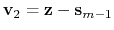 is the vector connecting the second closest frame to the current position,
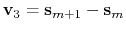 is the vector connecting the closest frame to the third closest frame, and
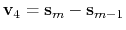 is the vector connecting the second closest frame to the closest frame.
and
is the vector connecting the second closest frame to the closest frame.
and  are the current index of the closest frame and the total number of frames, respectively. If the current position is on the left of the closest reference frame, the
  in
turns to the positive sign. Otherwise it turns to the negative sign.
in
turns to the positive sign. Otherwise it turns to the negative sign.
The equations above assume: (i) the frames are equidistant and (ii) the second and the third closest frames are neighbouring to the closest frame. When these assumptions are not satisfied, this set of path CV should be used carefully.
gspath: progress along a path defined in atomic Cartesian coordinate space.
In the gspath {...} and the gzpath {...} block all vectors, namely
 and
and
 are defined in atomic Cartesian coordinate space. More specifically,
![$ \mathbf{z} = \left[\mathbf{r}_{1}, \cdots, \mathbf{r}_{n}\right]$](img372.png) , where
, where
 is the
-th atom specified in the atoms block.
is the
-th atom specified in the atoms block.
![$ \mathbf{s}_{k} = \left[\mathbf{r}_{k,1}, \cdots, \mathbf{r}_{k,n}\right]$](img374.png) , where
, where
 means the
-th atom of the
means the
-th atom of the  -th reference frame.
List of keywords (see also 9.3.15 for additional options):
- atoms
Group of atoms
Context: gspath and gzpath
Acceptable Values: Block atoms {...}
Description: Defines the atoms whose coordinates make up the value of the component.
- refPositionsCol
PDB column containing atom flags
Context: gspath and gzpath
Acceptable Values: O, B, X, Y, or Z
Description: If refPositionsFileN is a PDB file that contains all the atoms in the topology, this option may be provided to set which PDB field is used to flag the reference coordinates for atoms.
- refPositionsFileN
File containing the reference positions for fitting
Context: gspath and gzpath
Acceptable Values: UNIX filename
Description: The path is defined by multiple refPositionsFiles which are similiar to refPositionsFile in the rmsd CV. If your path consists of  nodes, you can list the coordinate file (in PDB or XYZ format) from refPositionsFile1 to refPositionsFile10.
- useSecondClosestFrame
Define
 as the second closest frame?
Context: gspath and gzpath
Acceptable Values: boolean
Default Value: on
Description: The definition assumes the second closest frame is neighbouring to the closest frame. This is not always true especially when the path is crooked. If this option is set to on (default),
is defined as the second closest frame. If this option is set to off,
is defined as the left or right neighbouring frame of the closest frame.
- useThirdClosestFrame
Define
 as the third closest frame?
Context: gspath and gzpath
Acceptable Values: boolean
Default Value: off
Description: The definition assumes the third closest frame is neighbouring to the closest frame. This is not always true especially when the path is crooked. If this option is set to on,
is defined as the third closest frame. If this option is set to off (default),
is defined as the left or right neighbouring frame of the closest frame.
- fittingAtoms
The atoms that are used for alignment
Context: gspath and gspath
Acceptable Values: Group of atoms
Description: Before calculating
 ,
,
 ,
,
 and
and
 , the current frame need to be aligned to the corresponding reference frames. This option specifies which atoms are used to do alignment.
gzpath: distance from a path defined in atomic Cartesian coordinate space.
List of keywords (see also 9.3.15 for additional options):
The usage of gzpath and gspath is illustrated below:
colvar {
# Progress along the path
name gs
# The path is defined by 5 reference frames (from string-00.pdb to string-04.pdb)
# Use atomic coordinate from atoms 1, 2 and 3 to compute the path
gspath {
atoms {atomnumbers { 1 2 3 }}
refPositionsFile1 string-00.pdb
refPositionsFile2 string-01.pdb
refPositionsFile3 string-02.pdb
refPositionsFile4 string-03.pdb
refPositionsFile5 string-04.pdb
}
}
colvar {
# Distance from the path
name gz
# The path is defined by 5 reference frames (from string-00.pdb to string-04.pdb)
# Use atomic coordinate from atoms 1, 2 and 3 to compute the path
gzpath {
atoms {atomnumbers { 1 2 3 }}
refPositionsFile1 string-00.pdb
refPositionsFile2 string-01.pdb
refPositionsFile3 string-02.pdb
refPositionsFile4 string-03.pdb
refPositionsFile5 string-04.pdb
}
}
linearCombination: Helper CV to define a linear combination of other CVs
This is a helper CV which can be defined as a linear combination of other CVs. It maybe useful when you want to define the gspathCV {...} and the gzpathCV {...} as combinations of other CVs.
gspathCV: progress along a path defined in CV space.
In the gspathCV {...} and the gzpathCV {...} block all vectors, namely
and
are defined in CV space. More specifically,
![$ \mathbf{z} = \left[{\xi}_{1}, \cdots, {\xi}_{n}\right]$](img385.png) , where
, where  is the
-th CV.
is the
-th CV.
![$ \mathbf{s}_{k} = \left[{\xi}_{k,1}, \cdots, {\xi}_{k,n}\right]$](img387.png) , where
, where
 means the
-th CV of the
-th reference frame. It should be note that these two CVs requires the pathFile option, which specifies a path file. Each line in the path file contains a set of space-seperated CV value of the reference frame. The sequence of reference frames matches the sequence of the lines.
means the
-th CV of the
-th reference frame. It should be note that these two CVs requires the pathFile option, which specifies a path file. Each line in the path file contains a set of space-seperated CV value of the reference frame. The sequence of reference frames matches the sequence of the lines.
List of keywords (see also 9.3.15 for additional options):
gzpathCV: distance from a path defined in CV space.
List of keywords (see also 9.3.15 for additional options):
The usage of gzpathCV and gspathCV is illustrated below:
colvar {
# Progress along the path
name gs
# Path defined by the CV space of two dihedral angles
gspathCV {
pathFile ./path.txt
dihedral {
name 001
group1 {atomNumbers {5}}
group2 {atomNumbers {7}}
group3 {atomNumbers {9}}
group4 {atomNumbers {15}}
}
dihedral {
name 002
group1 {atomNumbers {7}}
group2 {atomNumbers {9}}
group3 {atomNumbers {15}}
group4 {atomNumbers {17}}
}
}
}
colvar {
# Distance from the path
name gz
gzpathCV {
pathFile ./path.txt
dihedral {
name 001
group1 {atomNumbers {5}}
group2 {atomNumbers {7}}
group3 {atomNumbers {9}}
group4 {atomNumbers {15}}
}
dihedral {
name 002
group1 {atomNumbers {7}}
group2 {atomNumbers {9}}
group3 {atomNumbers {15}}
group4 {atomNumbers {17}}
}
}
}
Arithmetic path collective variables
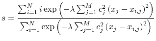
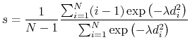
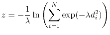
The arithmetic path collective variable in CV space uses the same formula as the one proposed by Branduardi[12] et al., except that it computes
and
in CV space instead of RMSDs in Cartesian space. Moreover, this implementation allows different coefficients for each CV components as described in [59]. Assuming a path is composed of
reference frames and defined in an
-dimensional CV space, then the equations of
and
of the path are
 |
(49) |
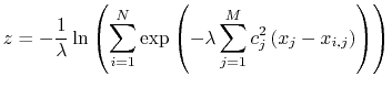 |
(50) |
where  is the coefficient(weight) of the
-th CV,
is the coefficient(weight) of the
-th CV,  is the value of
-th CV of
-th reference frame and
is the value of
-th CV of
-th reference frame and  is the value of
-th CV of current frame.
is the value of
-th CV of current frame.  is a parameter to smooth the variation of
and
.
is a parameter to smooth the variation of
and
.
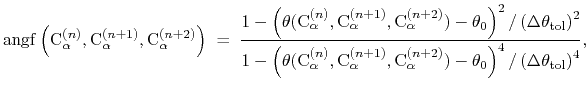
aspathCV: progress along a path defined in CV space.
This colvar component computes the
variable.
List of keywords (see also 9.3.15 for additional options):
azpathCV: distance from a path defined in CV space.
This colvar component computes the
variable. Options are the same as in 9.3.10.
The usage of azpathCV and aspathCV is illustrated below:
colvar {
# Progress along the path
name as
# Path defined by the CV space of two dihedral angles
aspathCV {
pathFile ./path.txt
weights {1.0 1.0}
lambda 0.005
dihedral {
name 001
group1 {atomNumbers {5}}
group2 {atomNumbers {7}}
group3 {atomNumbers {9}}
group4 {atomNumbers {15}}
}
dihedral {
name 002
group1 {atomNumbers {7}}
group2 {atomNumbers {9}}
group3 {atomNumbers {15}}
group4 {atomNumbers {17}}
}
}
}
colvar {
# Distance from the path
name az
azpathCV {
pathFile ./path.txt
weights {1.0 1.0}
lambda 0.005
dihedral {
name 001
group1 {atomNumbers {5}}
group2 {atomNumbers {7}}
group3 {atomNumbers {9}}
group4 {atomNumbers {15}}
}
dihedral {
name 002
group1 {atomNumbers {7}}
group2 {atomNumbers {9}}
group3 {atomNumbers {15}}
group4 {atomNumbers {17}}
}
}
}
Path collective variables in Cartesian coordinates
The path collective variables defined by Branduardi et al. [12]
are based on RMSDs in Cartesian coordinates.
Noting  the RMSD between the current set of Cartesian coordinates and those of image number
of the path:
the RMSD between the current set of Cartesian coordinates and those of image number
of the path:
 |
(51) |
 |
(52) |
where
is the smoothing parameter.
These coordinates are implemented as Tcl-scripted combinations of rmsd components.
The implementation is available as file colvartools/pathCV.tcl, and
an example is provided in file examples/10_pathCV.namd of the Colvars public repository.
It implements an optimization procedure, whereby the distance to a given image is only calculated if its contribution
to the sum is larger than a user-defined tolerance parameter.
All distances are calculated every freq timesteps to update the list of nearby images.
Volumetric map-based variables
Volumetric maps of the Cartesian coordinates, typically defined as mesh grid along the three Cartesian axes, may be used to define collective variables.
This feature is currently available in NAMD, implemented as an interface between Colvars and GridForces (see section 8).
Please cite [34] when using this implementation of collective variables based on volumetric maps.
mapTotal: total value of a volumetric map
Given a function of the Cartesian coordinates
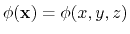 , a mapTotal collective variable component
 is defined as the sum of the values of the function
 evaluated at the coordinates of each atom,
 :
:
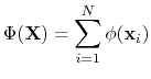 |
(53) |
This formulation allows, for example, to ``count'' the number of atoms within a region of space by using a positive-valued function
, such as for example the number of water molecules in a hydrophobic cavity [34].
Because the volumetric map itself and the atoms affected by it are defined externally to Colvars, this component has a very limited number of keywords.
List of keywords (see also 9.3.15 for additional options):
- mapName
Specify the name of the volumetric map to use as a colvar
Context: mapTotal
Acceptable Values: string
Description: The value of this option specifies the label of the volumetric map to use for this collective variable component.
This label must identify a map already loaded in NAMD via mGridForcePotFile, and its value of mGridForceScale needs to be set to (0, 0, 0), so that its collective force can be computed dynamically.
Example: biasing the number of molecules inside a cavity using a volumetric map.
Firstly, a volumetric map that has a value of 1 inside the cavity and 0 outside should be prepared.
A reasonable starting point may be obtained, for example, with VMD: using an existing trajectory where the cavity is occupied by solvent and a spatial selection that identifies all the molecules within the cavity, volmap occupancy -allframes -combine max computes the occupancy map as a step function (values 1 or 0), and volutil -smooth ... makes it a continuous map, suitable for use as a MD simulation bias.
A PDB file defining the selection (for example, where all water oxygens and ions have an occupancy of 1 and other atoms 0) is also prepared using VMD.
Both the map file and the atom selection file are then loaded via the mGridForcePotFile and related NAMD commands:
mGridForce yes
mGridForcePotFile Cavity cavity.dx # OpenDX map file
mGridForceFile Cavity water-sel.pdb # PDB file used for atom selection
mGridForceCol Cavity O # Use the occupancy column of the PDB file
mGridForceChargeCol Cavity B # Use beta as ``charge'' (default: electric charge)
mGridForceScale Cavity 0.0 0.0 0.0 # Do not use GridForces for this map
The value of mGridForceScale is particularly important, because it determines the GridForces force constant for the ``Cavity'' map.
A non-zero value enables a conventional GridForces calculation, where the force constant remains fixed within each run command and the forces on the atoms depend only on their positions in space.
However, setting mGridForceScale to zero signals to NAMD that the force acting through the volumetric map may be computed dynamically, as part of a collective-variable biasing scheme.
To do so, the map labeled ``Cavity'' needs to be referred to in the Colvars configuration:
cv config "
colvar {
name n_waters
mapTotal {
mapName Cavity # Same label as the GridForce map
}
}"
The variable ``n_waters'' may then be used with any of the enhanced sampling methods available (9.5): new forces applied to it at each simulation step will be transmitted to the corresponding atoms within the same step.
Multiple volumetric maps collective variables
To study processes that involve changes in shape of a macromolecular aggregate (for example, deformations of lipid membranes) it is useful to define collective variables based on more than one volumetric map at a time, measuring the relative similarity with each map while still achieving correct thermodynamic sampling of each state.
This is achieved by combining multiple mapTotal components, each based on a differently-shaped volumetric map, into a single collective variable
.
To track transitions between states, the contribution of each map to
should be discriminated from the others, for example by assigning to it a different weight.
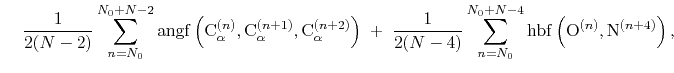
The ``Multi-Map'' progress variable [34] uses a weight sum of these components, using linearly-increasing weights:
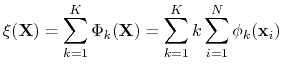 |
(54) |
where  is the number of maps employed and each
  is a mapTotal component.
Example: transitions between macromolecular shapes using volumetric maps.
A series of map files, each representing a different shape, is loaded into NAMD:
mGridForce yes
for { set k 1 } { $k <= $K } { incr k } {
mGridForcePotFile Shape_$k map_$k.dx # Density map of the k-th state
mGridForceFile Shape_$k atoms.pdb # PDB file used for atom selection
mGridForceCol Shape_$k O # Use the occupancy column of the PDB file atoms.pdb
mGridForceChargeCol Shape_$k B # Use beta as ``charge'' (default: electric charge)
mGridForceScale Shape_$k 0.0 0.0 0.0 # Do not use GridForces for this map
}
The GridForces maps thus loaded are then used to define the Multi-Map collective variable, with coefficients  [34]:
[34]:
# Collect the definition of all components into one string
set components "
for { set k 1 } { $k <= $K } { incr k } {
set components "${components}
mapTotal {
mapName Shape_$k
componentCoeff $k
}
"
}
# Use this string to define the variable
cv config "
colvar {
name shapes
${components}
}"
The above example illustrates a use case where a weighted sum (i.e. a linear combination) is used to define a single variable from multiple components.
Depending on the problem under study, non-linear functions may be more appropriate.
These may be defined a custom functions if implemented (see 9.3.16), or scripted functions (see 9.3.17).
Shared keywords for all components
The following options can be used for any of the above colvar components in order to obtain a polynomial combination or any user-supplied function provided by scriptedFunction (see 9.3.15).
- name
Name of this component
Context: any component
Acceptable Values: string
Default Value: type of component + numeric id
Description: The name is an unique case-sensitive string which allows the
Colvars module to identify this component. This is useful, for example,
when combining multiple components via a scriptedFunction.
It also defines the variable name representing the component's value in a customFunction (see 9.3.16) expression.
- scalable
Attempt to calculate this component in parallel?
Context: any component
Acceptable Values: boolean
Default Value: on, if available
Description: If set to on (default), the Colvars module will attempt to calculate this component in parallel to reduce overhead.
Whether this option is available depends on the type of component: currently supported are distance, distanceZ, distanceXY, distanceVec, distanceDir, angle and dihedral.
This flag influences computational cost, but does not affect numerical results: therefore, it should only be turned off for debugging or testing purposes.
Periodic components
The following components returns
real numbers that lie in a periodic interval:
- dihedral: torsional angle between four groups;
- spinAngle: angle of rotation around a predefined axis
in the best-fit from a set of reference coordinates.
In certain conditions, distanceZ can also be periodic, namely
when periodic boundary conditions (PBCs) are defined in the simulation
and distanceZ's axis is parallel to a unit cell vector.
In addition, a custom or scripted scalar colvar may be periodic
depending on its user-defined expression. It will only be treated as such by
the Colvars module if the period is specified using the period keyword,
while wrapAround is optional.
The following keywords can be used within periodic components, or within custom variables (9.3.16), or wthin scripted variables 9.3.17).
- period
Period of the component
Context: distanceZ, custom colvars
Acceptable Values: positive decimal
Default Value: 0.0
Description: Setting this number enables the treatment of distanceZ as
a periodic component: by default, distanceZ is not
considered periodic. The keyword is supported, but irrelevant
within dihedral or spinAngle, because their
period is always 360 degrees.
- wrapAround
Center of the wrapping interval for periodic variables
Context: distanceZ, dihedral, spinAngle, custom colvars
Acceptable Values: decimal
Default Value: 0.0
Description: By default, values of the periodic components are centered around zero, ranging from  to
to  , where
  is the period.
Setting this number centers the interval around this value.
This can be useful for convenience of output, or to set the walls for a harmonicWalls in an order that would not otherwise be allowed.
is the period.
Setting this number centers the interval around this value.
This can be useful for convenience of output, or to set the walls for a harmonicWalls in an order that would not otherwise be allowed.
Internally, all differences between two values of a periodic colvar
follow the minimum image convention: they are calculated based on
the two periodic images that are closest to each other.
Note: linear or polynomial combinations of periodic components (see 9.3.15) may become meaningless when components cross the periodic boundary. Use such combinations carefully: estimate the range of possible values of each component in a given simulation, and make use of wrapAround to limit this problem whenever possible.
Non-scalar components
When one of the following components are used, the defined colvar returns a value that is not a scalar number:
- distanceVec: 3-dimensional vector of the distance
between two groups;
- distanceDir: 3-dimensional unit vector of the distance
between two groups;
- orientation: 4-dimensional unit quaternion representing
the best-fit rotation from a set of reference coordinates.
The distance between two 3-dimensional unit vectors is computed as the
angle between them. The distance between two quaternions is computed
as the angle between the two 4-dimensional unit vectors: because the
orientation represented by
 is the same as the one
represented by
is the same as the one
represented by
 , distances between two quaternions are
computed considering the closest of the two symmetric images.
, distances between two quaternions are
computed considering the closest of the two symmetric images.
Non-scalar components carry the following restrictions:
- Calculation of total forces (outputTotalForce option)
is currently not implemented.
- Each colvar can only contain one non-scalar component.
- Binning on a grid (abf, histogram and
metadynamics with useGrids enabled) is currently
not implemented for colvars based on such components.
Note: while these restrictions apply to individual colvars based
on non-scalar components, no limit is set to the number of scalar
colvars. To compute multi-dimensional histograms and PMFs, use sets
of scalar colvars of arbitrary size.
Calculating total forces
In addition to the restrictions due to the type of value computed (scalar or non-scalar),
a final restriction can arise when calculating total force
(outputTotalForce option or application of a abf
bias). total forces are available currently only for the following
components: distance, distanceZ,
distanceXY, angle, dihedral, rmsd,
eigenvector and gyration.
Linear and polynomial combinations of components
To extend the set of possible definitions of colvars
 , multiple components
 can be summed with the formula:
![$\displaystyle \xi(\mathbf{r}) = \sum_i c_i [q_i(\mathbf{r})]^{n_i}$](img412.png) |
(55) |
where each component appears with a unique coefficient  (1.0 by
default) the positive integer exponent
(1.0 by
default) the positive integer exponent  (1 by default).
Any set of components can be combined within a colvar, provided that
they return the same type of values (scalar, unit vector, vector, or
quaternion). By default, the colvar is the sum of its components.
Linear or polynomial combinations (following
equation (56)) can be obtained by setting the
following parameters, which are common to all components:
Example: To define the average of a colvar across
different parts of the system, simply define within the same colvar
block a series of components of the same type (applied to different
atom groups), and assign to each component a componentCoeff
of  .
.
Custom functions
Collective variables may be defined by specifying a custom function as an analytical
expression.
The expression is parsed by Lepton, the lightweight expression parser written by Peter Eastman (https://simtk.org/projects/lepton).
Lepton produces efficient evaluation routines for the function and its derivatives.
The expression may use the collective variable components as variables, referred to by their user-defined name.
Scalar elements of vector components may be accessed by appending a 1-based index to their name, as in the example below.
When implementing generic functions of Cartesian coordinates rather
than functions of existing components, the cartesian component
may be particularly useful.
A scalar-valued custom variable may be manually defined as periodic by providing
the keyword period, and the optional keyword wrapAround, with the
same meaning as in periodic components (see 9.3.13 for details).
A vector variable may be defined by specifying the customFunction parameter several times: each expression defines one scalar element of the vector colvar, as in this example:
colvar {
name custom
# A 2-dimensional vector function of a scalar x and a 3-vector r
customFunction cos(x) * (r1 + r2 + r3)
customFunction sqrt(r1 * r2)
distance {
name x
group1 { atomNumbers 1 }
group2 { atomNumbers 50 }
}
distanceVec {
name r
group1 { atomNumbers 10 11 12 }
group2 { atomNumbers 20 21 22 }
}
}
Numeric constants may be given in either decimal or exponential form (e.g. 3.12e-2).
An expression may be followed by definitions for intermediate values that
appear in the expression, separated by semicolons.
For example, the expression:
a^2 + a*b + b^2; a = a1 + a2; b = b1 + b2
is exactly equivalent to:
(a1 + a2)^2 + (a1 + a2) * (b1 + b2) + (b1 + b2)^2.
The definition of an intermediate value may itself involve other intermediate values.
All uses of a value must appear before that value's definition.
Lepton supports the usual arithmetic operators +, -, *, /, and ^ (power), as well as the following functions:
| sqrt |
Square root |
| exp |
Exponential |
| log |
Natural logarithm |
| erf |
Error function |
| erfc |
Complementary error function |
| sin |
Sine (angle in radians) |
| cos |
Cosine (angle in radians) |
| sec |
Secant (angle in radians) |
| csc |
Cosecant (angle in radians) |
| tan |
Tangent (angle in radians) |
| cot |
Cotangent (angle in radians) |
| asin |
Inverse sine (in radians) |
| acos |
Inverse cosine (in radians) |
| atan |
Inverse tangent (in radians) |
| atan2 |
Two-argument inverse tangent (in radians) |
| sinh |
Hyperbolic sine |
| cosh |
Hyperbolic cosine |
| tanh |
Hyperbolic tangent |
| abs |
Absolute value |
| floor |
Floor |
| ceil |
Ceiling |
| min |
Minimum of two values |
| max |
Maximum of two values |
| delta |
 if
if  , 0 otherwise
 |
| step |
 if
if  , 1 if
|
| select |
 if
,
if
,  otherwise
 |
Scripted functions
When scripting is supported (default in NAMD),
a colvar may be defined as a scripted function of its components,
rather than a linear or polynomial combination.
When implementing generic functions of Cartesian coordinates rather
than functions of existing components, the cartesian component
may be particularly useful.
A scalar-valued scripted variable may be manually defined as periodic by providing
the keyword period, and the optional keyword wrapAround, with the
same meaning as in periodic components (see 9.3.13 for details).
An example of elaborate scripted colvar is given in example 10, in the
form of path-based collective variables as defined by Branduardi et al[12]
(Section 9.3.10).
- scriptedFunction
Compute colvar as a scripted function of its components
Context: colvar
Acceptable Values: string
Description: If this option is specified, the colvar will be computed as a
scripted function of the values of its components.
To that effect, the user should define two Tcl procedures:
calc_
scriptedFunction
and calc_
scriptedFunction
_gradient,
both accepting as many parameters as the colvar has components.
Values of the components will be passed to those procedures in the
order defined by their sorted name strings. Note that if all
components are of the same type, their default names are sorted in the
order in which they are defined, so that names need only be specified
for combinations of components of different types.
calc_
scriptedFunction
should return one value of
type
scriptedFunctionType
, corresponding to the colvar value.
calc_
scriptedFunction
_gradient should return a Tcl list
containing the derivatives of the function with respect to each
component.
If both the function and some of the components are vectors, the gradient
is really a Jacobian matrix that should be passed as a linear vector in
row-major order, i.e. for a function  :
:
 .
.
- scriptedFunctionType
Type of value returned by the scripted colvar
Context: colvar
Acceptable Values: string
Default Value: scalar
Description: If a colvar is defined as a scripted function, its type is not constrained by
the types of its components. With this flag, the user may specify whether the
colvar is a scalar or one of the following vector types: vector3
(a 3D vector), unit_vector3 (a normalized 3D vector), or
unit_quaternion (a normalized quaternion), or vector
(a vector whose size is specified by scriptedFunctionVectorSize).
Non-scalar values should be passed as space-separated lists.
- scriptedFunctionVectorSize
Dimension of the vector value of a scripted colvar
Context: colvar
Acceptable Values: positive integer
Description: This parameter is only valid when scriptedFunctionType is
set to vector. It defines the vector length of the colvar value
returned by the function.
Defining grid parameters
Many algorithms require the definition of boundaries and/or characteristic spacings that can be used to define discrete ``states'' in the collective variable, or to combine variables with very different units.
The parameters described below offer a way to specify these parameters only once for each variable, while using them multiple times in restraints, time-dependent biases or analysis methods.
- width
Unit of the variable, or grid spacing
Context: colvar
Acceptable Values: positive decimal
Default Value: 1.0
Description: This number defines the effective unit of measurement for the collective variable, and is used by the biasing methods for the following purposes.
Harmonic (9.5.5), harmonic walls (9.5.7) and linear restraints (9.5.8) use it to set the physical unit of the force constant, which is useful for multidimensional restraints involving multiple variables with very different units (for examples,  or degrees
) with a single, scaled force constant.
The values of the scaled force constant in the units of each variable are printed at initialization time.
Histograms (9.5.10), ABF (9.5.2) and metadynamics (9.5.4) all use this number as the initial choice for the grid spacing along this variable: for this reason, width should generally be no larger than the standard deviation of the colvar in an unbiased simulation.
Unless it is required to control the spacing, it is usually simplest to keep the default value of 1, so that restraint force constants are provided with their full physical unit.
or degrees
) with a single, scaled force constant.
The values of the scaled force constant in the units of each variable are printed at initialization time.
Histograms (9.5.10), ABF (9.5.2) and metadynamics (9.5.4) all use this number as the initial choice for the grid spacing along this variable: for this reason, width should generally be no larger than the standard deviation of the colvar in an unbiased simulation.
Unless it is required to control the spacing, it is usually simplest to keep the default value of 1, so that restraint force constants are provided with their full physical unit.
- lowerBoundary
Lower boundary of the colvar
Context: colvar
Acceptable Values: decimal
Default Value: natural boundary of the function
Description: Defines the lowest end of the interval of ``relevant'' values for the variable.
This number can be, for example, a true physical boundary imposed by the choice of function (e.g. the distance function is always larger than zero): if this is the case, and only one function is used to define the variable, the default value of this number is set to the lowest end of the range of values of that function, if available (see Section 9.3.1).
Alternatively, this value may be provided by the user, to represent for example the left-most point of a PMF calculation along this variable.
In the latter case, it is the user's responsibility to either (a) ensure the variable does not go significantly beyond the boundary (for example by adding a harmonicWalls restraint, 9.5.7), or (b) instruct the code that this is a true physical boundary by setting hardLowerBoundary (see 9.3.18).
- upperBoundary
Upper boundary of the colvar
Context: colvar
Acceptable Values: decimal
Default Value: natural boundary of the function
Description: Similarly to lowerBoundary, defines the highest of the ``relevant'' values of the variable.
- hardLowerBoundary
Whether the lower boundary is the physical lower limit
Context: colvar
Acceptable Values: boolean
Default Value: provided by the component
Description: When the colvar has a ``natural'' boundary (for example, a distance colvar cannot go below 0) this flag is automatically enabled.
For more complex variable definitions, or when lowerBoundary (see 9.3.18) is provided directly by the user, it may be useful to set this flag explicitly.
This option does not affect simulation results, but enables some internal optimizations by letting the code know that the variable is unable to cross the lower boundary, regardless of whether restraints are applied to it.
- hardUpperBoundary
Whether the upper boundary is the physical upper limit of the colvar's values
Context: colvar
Acceptable Values: boolean
Default Value: provided by the component
Description: Analogous to hardLowerBoundary.
- expandBoundaries
Allow to expand the two boundaries if needed
Context: colvar
Acceptable Values: boolean
Default Value: off
Description: If defined, lowerBoundary and upperBoundary may be automatically expanded to accommodate colvar values that do not fit in the initial range.
Currently, this option is used by the metadynamics bias
(9.5.4) to keep all of its hills fully within
the grid. This option cannot be used when
the initial boundaries already span the full period of a periodic
colvar.
Grid files: multicolumn text format
Many simulation methods and analysis tools write files that contain functions of the collective variables tabulated on a grid (e.g. potentials of mean force or multidimentional histograms) for the purpose of analyzing results.
Such files are produced by ABF (9.5.2), metadynamics (9.5.4), multidimensional histograms (9.5.10), as well as any restraint with optional thermodynamic integration support (9.5.1).
In some cases, these files may also be read as input of a new simulation.
Suitable input files for this purpose are typically generated as output files of previous simulations, or directly by the user in the specific case of ensemble-biased metadynamics (9.5.4).
This section explains the ``multicolumn'' format used by these files.
For a multidimensional function  ,
,  , ...
, ... the multicolumn grid format is defined as follows:
| # |

|
|
|
|
|
|
| # |

|

|

|
|
|
|
| # |

|

|

|
|
|
|
| # |
... |
... |
... |
... |
|
|
| # |

|

|
|
|
|
|
| |
|
|
|
|
|
|
| |

|

|
... |

|
f(
,
, ...,
) |
|
| |
|
|
... |

|
f(
,
, ...,
) |
|
| |
... |
... |
... |
... |
... |
|
| |
|
|
|
|
|
|
Lines beginning with the character ``#'' are the header of the file.
is the number of collective variables sampled by the grid.
For each variable  ,
,
 is the lowest value sampled by the grid (i.e. the left-most boundary of the grid along
),
is the lowest value sampled by the grid (i.e. the left-most boundary of the grid along
),
 is the width of each grid step along
,
is the width of each grid step along
,
 is the number of points and
 is a flag whose value is 1 or 0 depending on whether the grid is periodic along
.
In most situations:
is a flag whose value is 1 or 0 depending on whether the grid is periodic along
.
In most situations:
-
is given by the lowerBoundary (see 9.3.18) keyword of the variable
;
-
is given by the width (see 9.3.18) keyword;
-
is calculated from the two above numbers and the upperBoundary (see 9.3.18) keyword;
-
is set to 1 if and only if
is periodic and the grids' boundaries cover its period.
Exception: there is a slightly different header in PMF files computed by ABF (9.5.2) or by other biases with an optional thermodynamic integration (TI) estimator (9.5.1).
In this case, free-energy gradients are accumulated on an (npoints)-long grid along each variable
: after these gradients are integrated, the resulting PMF is discretized on a grid with (npoints+1) points along
.
Therefore, the edges of the PMF's grid extend
 above and below the original boundaries (unless these are periodic). The format of the file's header is otherwise unchanged.
After the header, the rest of the file contains values of the tabulated function
,
, ...
 , one for each line.
The first
columns contain values of
, one for each line.
The first
columns contain values of  ,
, ...
,
, ...
 and the last column contains the value of the function
  .
Points are sorted in ascending order with the fastest-changing values at the right (``C-style'' order).
Each sweep of the right-most variable
is terminated by an empty line.
For two dimensional grid files, this allows quick visualization by programs such as GNUplot.
.
Points are sorted in ascending order with the fastest-changing values at the right (``C-style'' order).
Each sweep of the right-most variable
is terminated by an empty line.
For two dimensional grid files, this allows quick visualization by programs such as GNUplot.
Example 1: multicolumn text file for a one-dimensional histogram with lowerBoundary = 15, upperBoundary = 48 and width = 0.1.
| # |
1 |
|
|
|
|
| # |
15 |
0.1 |
330 |
0 |
|
| |
|
|
|
|
|
| |
15.05 |
6.14012e-07 |
|
|
|
| |
15.15 |
7.47644e-07 |
|
|
|
| |
... |
... |
|
|
|
| |
47.85 |
1.65944e-06 |
|
|
|
| |
47.95 |
1.46712e-06 |
|
|
|
| |
|
|
|
|
|
Example 2: multicolumn text file for a two-dimensional histogram of two dihedral angles (periodic interval with 6
bins):
| |
|
|
|
|
|
| # |
2 |
|
|
|
|
| # |
-180.0 |
6.0 |
30 |
1 |
|
| # |
-180.0 |
6.0 |
30 |
1 |
|
| |
|
|
|
|
|
| |
-177.0 |
-177.0 |
8.97117e-06 |
|
|
| |
-177.0 |
-171.0 |
1.53525e-06 |
|
|
| |
... |
... |
... |
|
|
| |
-177.0 |
177.0 |
2.442956-06 |
|
|
| |
|
|
|
|
|
| |
-171.0 |
-177.0 |
2.04702e-05 |
|
|
| |
... |
... |
... |
|
|
Trajectory output
Extended Lagrangian
The following options enable extended-system
dynamics, where a colvar is coupled to an additional degree of freedom
(fictitious particle) by a harmonic spring.
This extended coordinate masks the colvar and replaces it transparently from
the perspective of biasing and analysis methods.
Biasing forces are then applied to the extended degree
of freedom, and the actual geometric colvar (function of Cartesian
coordinates) only feels the force from the harmonic spring.
This is particularly useful when combined with an abf (see 9.5.2) bias
to perform eABF simulations (9.5.3).
Note that for some biases (harmonicWalls (see 9.5.7), histogram (see 9.5.10)),
this masking behavior is controlled by the keyword bypassExtendedLagrangian (see 9.5).
Specifically for harmonicWalls, the default behavior is to bypass extended Lagrangian
coordinates and act directly on the actual colvars.
- extendedLagrangian
Add extended degree of freedom
Context: colvar
Acceptable Values: boolean
Default Value: off
Description: Adds a fictitious particle to be coupled to the colvar by a harmonic
spring. The fictitious mass and the force constant of the coupling
potential are derived from the parameters extendedTimeConstant
and extendedFluctuation, described below. Biasing forces on the
colvar are applied to this fictitious particle, rather than to the
atoms directly. This implements the extended Lagrangian formalism
used in some metadynamics simulations [49].
The energy associated with the extended degree of freedom is reported
along with bias energies
under the MISC title in NAMD's energy output.
- extendedFluctuation
Standard deviation between the colvar and the fictitious
particle (colvar unit)
Context: colvar
Acceptable Values: positive decimal
Description: Defines the spring stiffness for the extendedLagrangian
mode, by setting the typical deviation between the colvar and the extended
degree of freedom due to thermal fluctuation.
The spring force constant is calculated internally as
 ,
where
,
where  is the value of extendedFluctuation.
- extendedTimeConstant
Oscillation period of the fictitious particle (fs)
Context: colvar
Acceptable Values: positive decimal
Default Value: 200
Description: Defines the inertial mass of the fictitious particle, by setting the
oscillation period of the harmonic oscillator formed by the fictitious
particle and the spring. The period
should be much larger than the MD time step to ensure accurate integration
of the extended particle's equation of motion.
The fictitious mass is calculated internally as
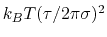 ,
where
,
where  is the period and
is the typical fluctuation (see above).
is the period and
is the typical fluctuation (see above).
- extendedTemp
Temperature for the extended degree of freedom (K)
Context: colvar
Acceptable Values: positive decimal
Default Value: thermostat temperature
Description: Temperature used for calculating the coupling force constant of the
extended variable (see extendedFluctuation) and, if needed, as a
target temperature for extended Langevin dynamics (see
extendedLangevinDamping). This should normally be left at its
default value.
- extendedLangevinDamping
Damping factor for extended Langevin dynamics
(ps
 )
)
Context: colvar
Acceptable Values: positive decimal
Default Value: 1.0
Description: If this is non-zero, the extended degree of freedom undergoes Langevin dynamics
at temperature extendedTemp. The friction force is minus
extendedLangevinDamping times the velocity. This is useful because
the extended dynamics coordinate may heat up in the transient
non-equilibrium regime of ABF. Use moderate damping values, to limit
viscous friction (potentially slowing down diffusive sampling) and stochastic
noise (increasing the variance of statistical measurements). In
doubt, use the default value.
Multiple time-step variables
- timeStepFactor
Compute this colvar once in a certain number of timesteps
Context: colvar
Acceptable Values: positive integer
Default Value: 1
Description: Instructs this colvar to activate at a time interval equal to the base (MD)
timestep times timeStepFactor.[32]
At other time steps, the value of the
variable is not updated, and no biasing forces are applied.
Any forces exerted by biases are accumulated over the given time interval,
then applied as an impulse at the next update.
Backward-compatibility
- subtractAppliedForce
Do not include biasing forces in the total force for this colvar
Context: colvar
Acceptable Values: boolean
Default Value: off
Description: If the colvar supports total force calculation (see 9.3.14), all forces applied to this colvar by biases will be removed from the total force.
This keyword allows to recover some of the ``system force'' calculation available in the Colvars module before version 2016-08-10.
Please note that removal of all other external forces (including biasing forces applied to a different colvar) is no longer supported, due to changes in the underlying simulation engines (primarily NAMD).
This option may be useful when continuing a previous simulation where the removal of external/applied forces is essential.
For all new simulations, the use of this option is not recommended.
Statistical analysis
Run-time calculations of statistical properties that depend explicitly on time can be performed for individual collective variables.
Currently, several types of time correlation functions, running averages and running standard deviations are implemented.
For run-time computation of histograms, please see the histogram bias (9.5.10).
- corrFunc
Calculate a time correlation function?
Context: colvar
Acceptable Values: boolean
Default Value: off
Description: Whether or not a time correlaction function should be calculated
for this colvar.
- corrFuncWithColvar
Colvar name for the correlation function
Context: colvar
Acceptable Values: string
Description: By default, the auto-correlation function (ACF) of this colvar,
, is calculated. When this option is specified, the
correlation function is calculated instead with another colvar,
 , which must be of the same type (scalar, vector, or
quaternion) as
.
, which must be of the same type (scalar, vector, or
quaternion) as
.
- corrFuncType
Type of the correlation function
Context: colvar
Acceptable Values: velocity, coordinate or
coordinate_p2
Default Value: velocity
Description: With coordinate or velocity, the correlation
function
 =
=
 is calculated between
the variables
and
, or their velocities.
is calculated between
the variables
and
, or their velocities.
 is the scalar product when calculated
between scalar or vector values, whereas for quaternions it is the
cosine between the two corresponding rotation axes. With
coordinate_p2, the second order Legendre polynomial,
is the scalar product when calculated
between scalar or vector values, whereas for quaternions it is the
cosine between the two corresponding rotation axes. With
coordinate_p2, the second order Legendre polynomial,
 , is used instead of the cosine.
- corrFuncNormalize
Normalize the time correlation function?
Context: colvar
Acceptable Values: boolean
Default Value: on
Description: If enabled, the value of the correlation function at  = 0
is normalized to 1; otherwise, it equals to
= 0
is normalized to 1; otherwise, it equals to
 .
.
- corrFuncLength
Length of the time correlation function
Context: colvar
Acceptable Values: positive integer
Default Value: 1000
Description: Length (in number of points) of the time correlation function.
- corrFuncStride
Stride of the time correlation function
Context: colvar
Acceptable Values: positive integer
Default Value: 1
Description: Number of steps between two values of the time correlation function.
- corrFuncOffset
Offset of the time correlation function
Context: colvar
Acceptable Values: positive integer
Default Value: 0
Description: The starting time (in number of steps) of the time correlation
function (default:
= 0). Note: the value at
= 0 is always
used for the normalization.
- corrFuncOutputFile
Output file for the time correlation function
Context: colvar
Acceptable Values: UNIX filename
Default Value: outputName.
name
.corrfunc.dat
Description: The time correlation function is saved in this file.
- runAve
Calculate the running average and standard deviation
Context: colvar
Acceptable Values: boolean
Default Value: off
Description: Whether or not the running average and standard deviation should
be calculated for this colvar.
- runAveLength
Length of the running average window
Context: colvar
Acceptable Values: positive integer
Default Value: 1000
Description: Length (in number of points) of the running average window.
- runAveStride
Stride of the running average window values
Context: colvar
Acceptable Values: positive integer
Default Value: 1
Description: Number of steps between two values within the running average window.
- runAveOutputFile
Output file for the running average and standard deviation
Context: colvar
Acceptable Values: UNIX filename
Default Value: outputName.
name
.runave.traj
Description: The running average and standard deviation are saved in this file.
Next: Selecting atoms
Up: Collective Variable-based Calculations (Colvars)
Previous: Enabling and controlling the
Contents
Index
http://www.ks.uiuc.edu/Research/namd/