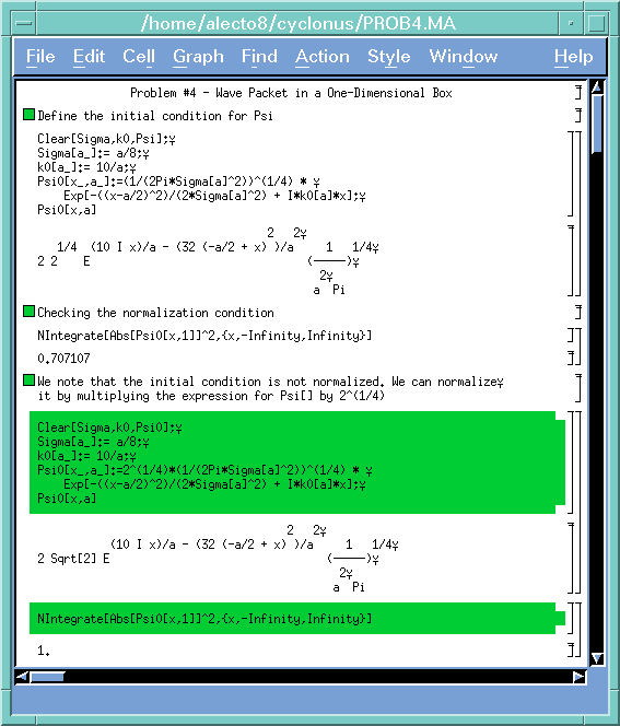
Here you'll find an example of how one can use Mathematica to handle messy algebraic manipulations. This notebook was written by one of the students in the class, who wishes to remain anonymous.
I don't know what the funny little symbols at the end of every lie are, but just ignore them. The initial wave function is called Psi0 in this notebook. The [x_,a_] mean the Psi0 is defined as a function of the variables x and a. We start by correcting a small mistake, namely that the initial wave function as given was not normalized to unity.

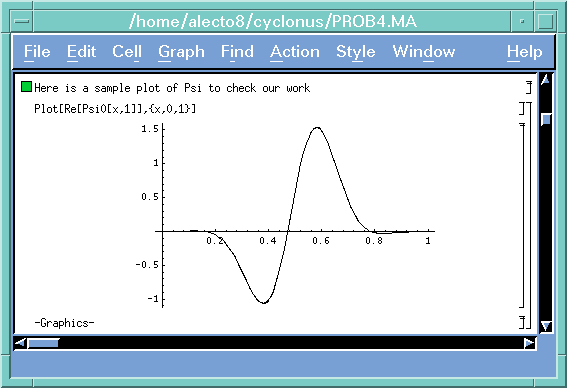
Notice that the following plot of the real part of the initial condition has a node at the center, while the probability |psi}^2 does not. Notice, too, that the peak of this real part higher than one, even though the probability density of course cannot be greater than one. This happens because the imaginary part of the wave function cancels out part of the real part, so that the norm squared looks like a Gaussian.
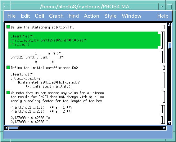
Now we define the stationary states of the square well as functions of x, a, and n, just as they were defined in class. Cn0, our expansion coefficients, are defined implicitly as a function of n, x, and a. Of course, x is just a dummy integration variable and could have been left out of the definition. It is also pointed out that the coefficients don't depend on the value of a. This may seem strange until you realize that all the parameters in the initial wave function, i.e. sigma, k0, and the center of the peak, were defined in terms of a. That means that no matter what value a takes, the initial wave function has the same shape relative to the shape of the stationary states, which are also scaled with a. Hence the results of all our integrals to calculate the Cn0's don't have a in the answer.
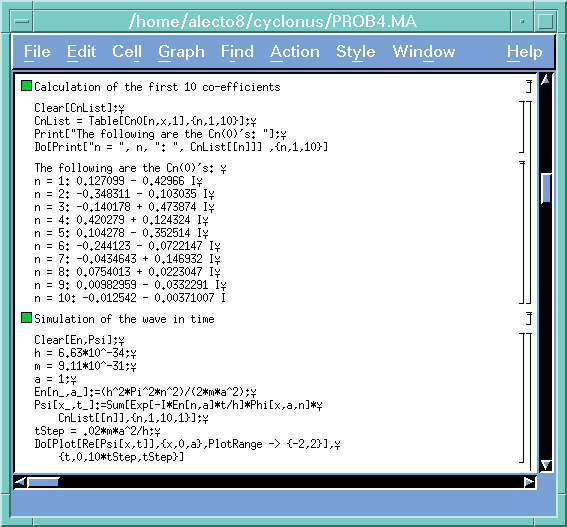
Now the real fun: we loop n from 1 to 10 and have Mathematica spit out the first ten coefficients for us. You don't have to use Mathematica to do this; Mathematica's strong suit isn't so much the numerical integration as the ability to set up problems like this with a minimum of fuss and get out meaningful results.
If you would like to explore further with with this notebook, you can download it here. Save it in your directory, and execute it with the command
mathematica PROB4.MA -displayFor more information about using Mathematica, you can also visit this site.:0.0 &