Electrostatic interactions between QM and MM atoms deserve a more detailed discussion due to the abundance and diversity of available alternatives. The first decision to be made is whether there will be electrostatic interactions between the two portions of a system, QM and MM. In the ``mechanical embedding" scheme, only positions and elements of atoms in the QM region are passed on to the chosen QC software for energy and force calculations. This way, QM and MM atoms share only van der Waals interactions.
|
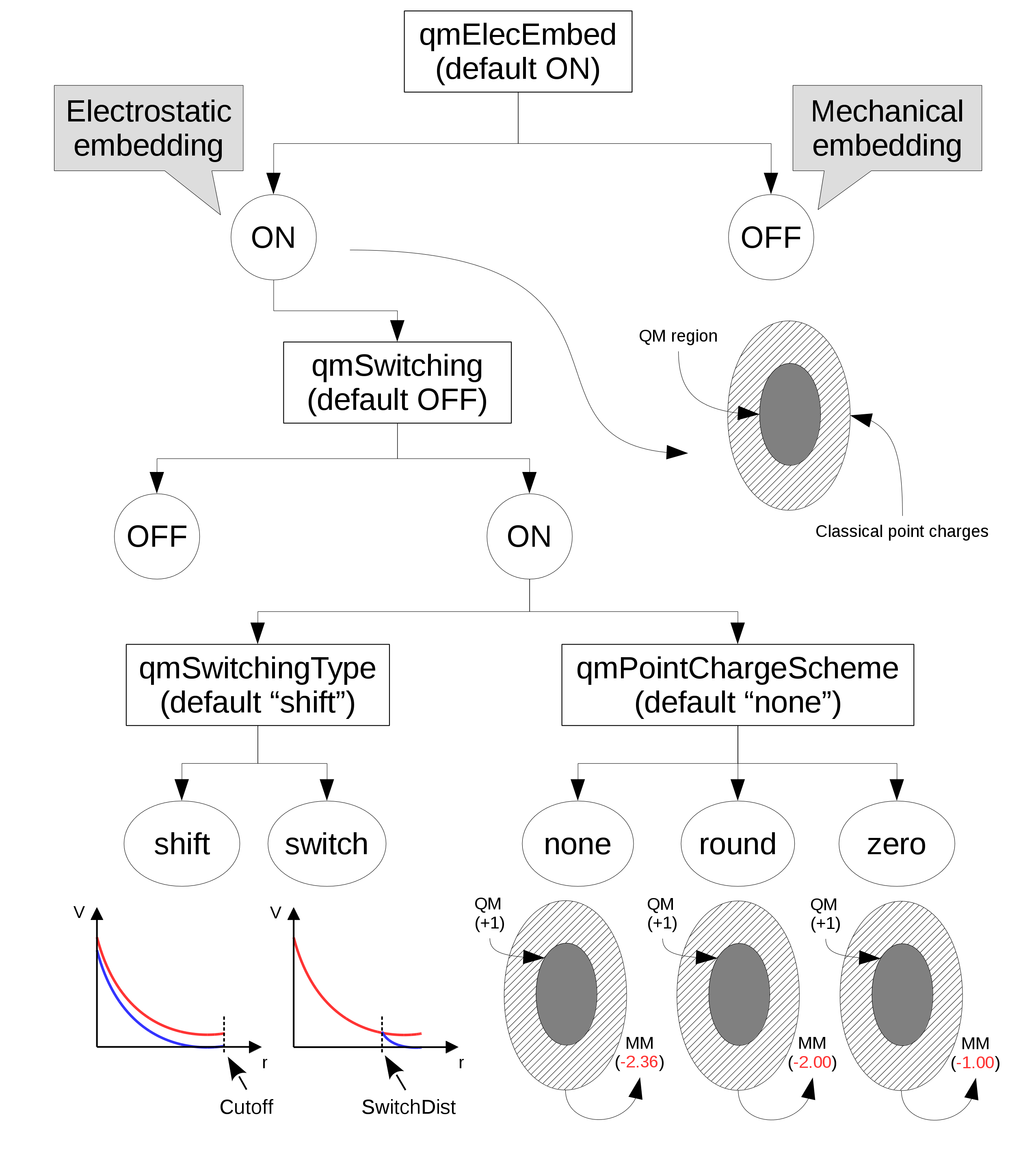
In the ``electrostatic embedding" scheme, on the other hand, the partial charges of MM atoms surrounding all QM atoms are used to approximate the electrostatic environment where QM atoms are found (the scheme is selected with the ``qmElecEmbed" keyword). See Figure 15. This process can be customized in a variety of ways, the first of which is deciding if a smoothing function will be used to avoid an abrupt decay in electrostatic force due to the cutoff used in the selection of surrounding point charges (this option is activated with the ``qmSwitching" keyword).
Classical point charge utilization can be further customized by choosing which smoothing function will be used, and if the total charge of selected partial charges should be modified to (A) have a whole charge or (B) have a complementary charge to that of the QM region, so that the sum of charges from QM atoms and classical partial charges add to zero (see Figure 15).
With electrostatic embedding, QM atoms are influenced by the charges in the classical region. In order to balance the forces acting on the system, NAMD uses partial charges for the QM atoms to calculate the electrostatic interaction with classical point charges. There are two possibilities for the origin of the QM partial charges: the original partial charges found in the force field parameter files can be used, or updated partial charges can be gathered at each step from the QC software output (controllable through the ``qmChargeMode" keyword). The continuous update in charge distribution allows for a partial re-parameterization of the targeted molecule at each time step, which can lead to an improved description of the interactions of a ligand as it repositions over the surface of a protein, for example, or as it moves through a membrane.
In case PME is activated by the user, NAMD will automatically apply the necessary corrections to handle the QM region, allowing it to be influenced by long range interactions from the entire system.